4 · Elastostatics as a Minimization Problem

Posing an elastic object is an optimization: pin part of the shape, drag a handle, and let everything else settle at the vertex positions \(x\) that minimize the energy below. The pin and handle terms are quadratic spring penalties of stiffness \(K\). We minimize with Newton (how that solve works is tutorial 5’s job) and focus on how different energies pose differently.

\[ E(x) = \underbrace{E_{\text{elastic}}(x)}_{\text{wants rest shape}} + \underbrace{\tfrac{K}{2}\lVert x_{\text{pin}} - p\rVert^2}_{\text{hold pins}} + \underbrace{\tfrac{K}{2}\lVert x_{\text{handle}} - h\rVert^2}_{\text{drag handle}}. \]

Imports, and every tunable parameter of this notebook.

%matplotlib inline
import os
import numpy as np
import matplotlib.pyplot as plt
import igl
import simkit
import utils

NOTEBOOK = "004_elastostatics_minimization"                        # this file's name
RESULTS_DIR = utils.notebook_results_path(NOTEBOOK)               # results/004_elastostatics_minimization/
MEDIA_DIR = "media"                                                # tracked copies for the website
# material and springs
MU, LAM = 1.0, 1.0                              # Lame parameters, the same on every element
K_PIN = 1e5                                     # stiffness of the pin and handle springs
POSE_MATERIAL = "macklin-mueller-neo-hookean"   # simkit material of both animations
MATERIALS = {"Linear": "linear-elasticity",     # plot label -> simkit material, for the comparison
             "ARAP": "arap",
             "Neo-Hookean": "macklin-mueller-neo-hookean"}
# solver and checks
NEWTON_ITERS = 100                              # max Newton iterations per pose
NEWTON_TOL = 1e-6                               # stop when the Newton step is shorter than this
FD_STEP = 1e-6                                  # central-difference step of the gradient check
FD_NOISE = 0.1                                  # size of the random deformation the check runs at
SEED = 0                                        # seed of that random deformation
# triangle experiments
N_FRAMES = 48                                   # handle positions per animation
FIG8_AMP = (0.45, 0.6)                          # figure-8 half-width (x) and half-height (y)
FAR_TARGET = np.array([1.5, 1.1])               # handle target of the material comparison
# beam experiment
NX, NY = 16, 5                                  # grid resolution (vertices)
WIDTH, HEIGHT = 2.0, 0.4                        # beam size
SWING_DEG = 120                                 # largest swing angle of the right edge
FPS = 20                                        # video frame rate

The posing system

elastic_pose_system builds the three terms of \(E(x)\) from simkit: the elastic material (evaluated on \(F = Jx\) with the deformation Jacobian \(J\) and weighted by element area), and two simkit.dirichlet_penalty quadratics for the fixed pin and the movable handle. It returns the energy, gradient and Hessian closures Newton needs, each summing its terms one per line (the Hessian is PSD-projected so Newton always goes downhill). Re-aiming the handle just means building the system again; every later tutorial builds its simulator this way.

def elastic_pose_system(X, T, material, pin_idx, pin_targets, handle_idx, handle_targets):
    """Elastic energy + a soft pin + a soft handle, in stacked vertex positions x."""
    n, dim = X.shape
    J = simkit.deformation_jacobian(X, T)
    vol = simkit.volume(X, T)
    mu = np.full((len(T), 1), MU)
    lam = np.full((len(T), 1), LAM)
    Q_pin, b_pin = simkit.dirichlet_penalty(pin_idx, pin_targets, n, K_PIN)
    Q_handle, b_handle = simkit.dirichlet_penalty(handle_idx, handle_targets, n, K_PIN)

    def energy_func(x):
        E_elastic = simkit.energies.elastic_energy_x(x.reshape(n, dim), J, mu, lam, vol, material)
        E_pin = simkit.energies.quadratic_energy(x, Q_pin, b_pin)
        E_handle = simkit.energies.quadratic_energy(x, Q_handle, b_handle)
        E_total = E_elastic + E_pin + E_handle
        return E_total

    def gradient_func(x):
        g_elastic = simkit.energies.elastic_gradient_x(x.reshape(n, dim), J, mu, lam, vol, material)
        g_pin = simkit.energies.quadratic_gradient(x, Q_pin, b_pin)
        g_handle = simkit.energies.quadratic_gradient(x, Q_handle, b_handle)
        g_total = g_elastic + g_pin + g_handle
        return g_total

    def hessian_func(x):
        H_elastic = simkit.energies.elastic_hessian_x(x.reshape(n, dim), J, mu, lam, vol, material, psd=True)
        H_pin = simkit.energies.quadratic_hessian(Q_pin)
        H_handle = simkit.energies.quadratic_hessian(Q_handle)
        H_total = H_elastic + H_pin + H_handle
        return H_total

    return energy_func, gradient_func, hessian_func

Two meshes

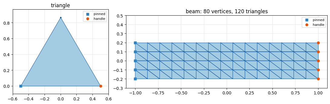
A single equilateral triangle (pin vertex 0, handle vertex 1) and a 16 × 5 cantilever beam from igl.triangulated_grid, centered and scaled (pin the whole left edge, the whole right edge is the handle). Blue squares mark pinned vertices, orange dots mark handles.

X_tri = np.array([[-0.5, 0.0], [0.5, 0.0], [0.0, np.sqrt(3) / 2]])
T_tri = np.array([[0, 1, 2]])
tri_pin, tri_handle = np.array([0]), np.array([1])

V, T_beam = igl.triangulated_grid(NX, NY)                      # unit square, NX x NY vertices
X_beam = (V - 0.5) * np.array([WIDTH, HEIGHT])                 # centered WIDTH x HEIGHT rectangle
beam_pin = np.where(X_beam[:, 0] <= X_beam[:, 0].min() + 1e-6)[0]
beam_handle = np.where(X_beam[:, 0] >= X_beam[:, 0].max() - 1e-6)[0]

fig, axes = plt.subplots(1, 2, figsize=(11, 3.4), gridspec_kw={"width_ratios": [1, 2.1]})
utils.plot_mesh(axes[0], X_tri, T_tri, pins=tri_pin, handles=tri_handle, title="triangle", show_vertices=True)
utils.plot_mesh(axes[1], X_beam, T_beam, pins=beam_pin, handles=beam_handle, lims=((-1.1, 1.1), (-0.3, 0.5)),
                title=f"beam: {len(X_beam)} vertices, {len(T_beam)} triangles")
fig.tight_layout()
simkit.filesystem.save_figure(fig, os.path.join(RESULTS_DIR, "meshes.png"),
                              copy_to=os.path.join(MEDIA_DIR, "004_meshes.png"))
plt.show()

Check the gradient

Before posing anything, compare gradient_func with central finite differences (simkit.gradient_cfd) of energy_func at a random deformation of the triangle, for each material, with the pin and handle aimed at their rest positions so all three terms are active. Relative errors around \(10^{-10}\) mean the energy and gradient are consistent, which Newton and its line search rely on.

rng = np.random.default_rng(SEED)
x_test = (X_tri + FD_NOISE * rng.standard_normal(X_tri.shape)).reshape(-1, 1)
for label, material in MATERIALS.items():
    energy_func, gradient_func, hessian_func = elastic_pose_system(
        X_tri, T_tri, material, tri_pin, X_tri[tri_pin], tri_handle, X_tri[tri_handle])
    g = gradient_func(x_test)
    g_fd = simkit.gradient_cfd(lambda y: np.array(energy_func(y.reshape(-1, 1))), x_test.ravel(), FD_STEP)
    rel_err = np.linalg.norm(g_fd.reshape(-1, 1) - g) / np.linalg.norm(g)
    print(f"{label:12s} |g_fd - g| / |g| = {rel_err:.1e}")

Linear       |g_fd - g| / |g| = 2.6e-10
ARAP         |g_fd - g| / |g| = 4.0e-10
Neo-Hookean  |g_fd - g| / |g| = 4.4e-10

A triangle: pin the left vertex, swing the right one in a figure-8

The handle traces a figure-8 (a lemniscate), so the free apex both stretches and compresses. At each handle position we build the system with the new target and re-solve, starting from the previous equilibrium. The × is the handle’s target, the orange dot where the handle vertex actually settles.

t = np.linspace(0, 2 * np.pi, N_FRAMES)
handle_path = X_tri[tri_handle] + np.stack([FIG8_AMP[0] * np.sin(t), FIG8_AMP[1] * np.sin(2 * t)], axis=1)

tri_states = []
U = X_tri.copy()
for h in handle_path:
    energy_func, gradient_func, hessian_func = elastic_pose_system(
        X_tri, T_tri, POSE_MATERIAL, tri_pin, X_tri[tri_pin], tri_handle, h[None])
    x = simkit.solvers.newton_solver(U.reshape(-1, 1), energy_func, gradient_func, hessian_func,
                                     tolerance=NEWTON_TOL, max_iter=NEWTON_ITERS, do_line_search=True)
    U = x.reshape(-1, 2)
    tri_states.append(U)

fig, anim = utils.animate_mesh(tri_states, T_tri, lims=((-1.2, 1.6), (-1.2, 1.2)),
    title="Neo-Hookean triangle: handle traces a figure-8",
    pin_pts=X_tri[tri_pin], handle_traj=[s[tri_handle] for s in tri_states],
    target_pts=list(handle_path), fps=FPS, figsize=(6, 5))
video = simkit.filesystem.save_animation(anim, os.path.join(RESULTS_DIR, "triangle.mp4"), fps=FPS,
                                         copy_to=os.path.join(MEDIA_DIR, "004_triangle.mp4"))
plt.close(fig)
utils.embed_video(video)

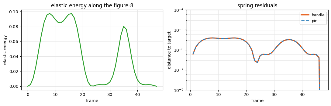
Per frame: the elastic energy of each equilibrium (left), highest on the stretching right lobe of the figure-8 (frames 1-23) and lower on the compressing left lobe (frames 24-46), and how far the pin and handle vertices sit from their targets (right). Soft springs never hold exactly; they stretch by about \(\lVert\nabla E_{\text{elastic}}\rVert / K\), a few \(10^{-6}\) here (zero at rest). The two curves coincide because the elastic forces on a triangle sum to zero, so both springs pull equally hard.

mu_tri = np.full((len(T_tri), 1), MU)
lam_tri = np.full((len(T_tri), 1), LAM)
tri_elastic = [simkit.energies.elastic_energy(X_tri, T_tri, mu_tri, lam_tri, POSE_MATERIAL, U) for U in tri_states]
tri_residuals = {
    "handle": [np.linalg.norm(U[tri_handle] - h[None], axis=1).max() for U, h in zip(tri_states, handle_path)],
    "pin": [np.linalg.norm(U[tri_pin] - X_tri[tri_pin], axis=1).max() for U in tri_states],
}
fig, axes = plt.subplots(1, 2, figsize=(11, 3.6))
frames = np.arange(N_FRAMES)
utils.line_plot(frames, {"Neo-Hookean": tri_elastic}, xlabel="frame", ylabel="elastic energy", ax=axes[0],
                title="elastic energy along the figure-8")
utils.residual_plot(tri_residuals, frames, ax=axes[1], colors={"handle": utils.HANDLE_C, "pin": utils.PIN_C},
                    xlabel="frame", ylabel="distance to target", title="spring residuals", ylim=(1e-8, 1e-4))
fig.tight_layout()
simkit.filesystem.save_figure(fig, os.path.join(RESULTS_DIR, "triangle_energy.png"),
                              copy_to=os.path.join(MEDIA_DIR, "004_triangle_energy.png"))
plt.show()

Same handle, three energies, very different poses

Pull the handle far up and to the right, and compare where the free apex lands under each model (dashed: rest shape, ×: handle target). We solve once per material from the rest shape, keeping each solve’s per-iteration gradients (return_info=True) for the convergence plot below.

fig, axes = plt.subplots(1, 3, figsize=(12, 4))
newton_grad_norms = {}
for ax, (label, material) in zip(axes, MATERIALS.items()):
    energy_func, gradient_func, hessian_func = elastic_pose_system(
        X_tri, T_tri, material, tri_pin, X_tri[tri_pin], tri_handle, FAR_TARGET[None])
    x, info = simkit.solvers.newton_solver(X_tri.reshape(-1, 1), energy_func, gradient_func, hessian_func,
                                           tolerance=NEWTON_TOL, max_iter=NEWTON_ITERS, do_line_search=True,
                                           return_info=True)
    newton_grad_norms[label] = [np.linalg.norm(g) for g in info["g"]] + [np.linalg.norm(gradient_func(x))]
    U = x.reshape(-1, 2)
    utils.setup_axes(ax, (-1.0, 2.0), (-0.8, 1.6), title=label)
    utils.TriangleArtist(ax, U, rest=X_tri)
    ax.plot(*X_tri[tri_pin[0]], "s", color=utils.PIN_C, ms=10)
    ax.plot(*FAR_TARGET, "x", color="0.3", ms=12, mew=2.5)
    print(f"{label:12s} free apex at ({U[2, 0]:+.2f}, {U[2, 1]:+.2f}), {len(info['g'])} Newton iterations")
fig.suptitle("Same pin + handle target, three elastic energies")
fig.tight_layout()
simkit.filesystem.save_figure(fig, os.path.join(RESULTS_DIR, "materials.png"),
                              copy_to=os.path.join(MEDIA_DIR, "004_materials.png"))
plt.show()

Linear       free apex at (-0.45, +1.13), 2 Newton iterations
ARAP         free apex at (+0.08, +1.31), 5 Newton iterations
Neo-Hookean  free apex at (+0.19, +1.11), 4 Newton iterations

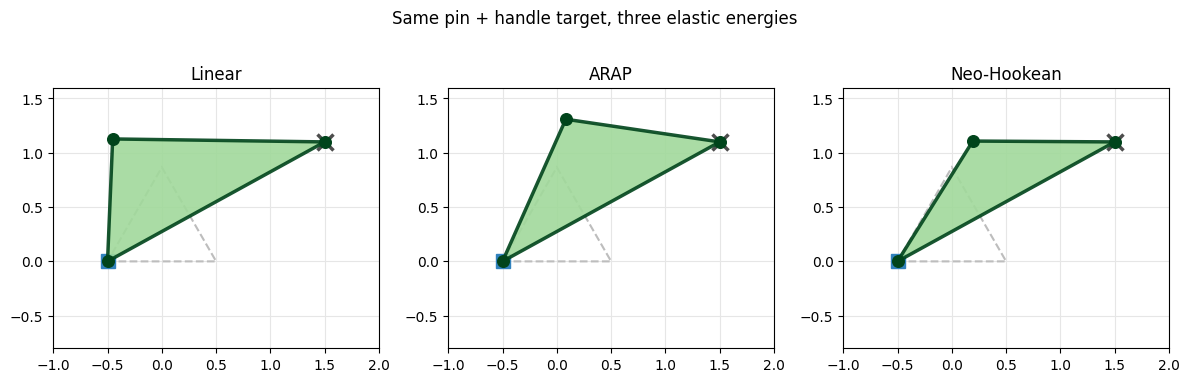
Linear elasticity is not rotation-invariant: it counts the large rotation this pose needs as strain, so it poses a lopsided triangle, unlike the two rotation-invariant models ARAP and Neo-Hookean.

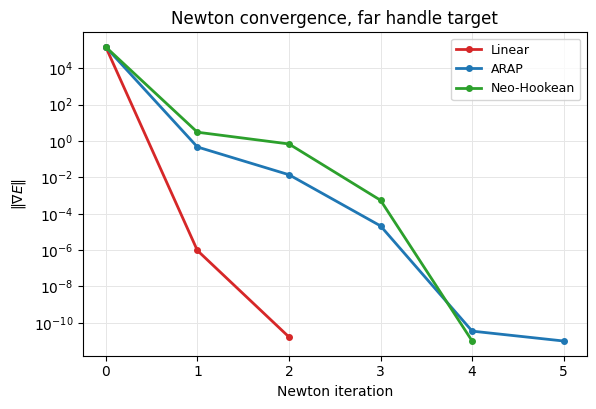
Gradient norm \(\lVert\nabla E\rVert\) per Newton iteration for those three solves. It starts at \(K \lVert h - x_{\text{handle}}\rVert \approx 1.5 \times 10^5\) (the handle spring’s pull) and falls by about 16 orders of magnitude in 2 to 5 iterations. Linear elasticity is quadratic, so its first step already lands on the minimum up to roundoff; the others end with Newton’s fast local convergence (tutorial 5).

fig, ax = utils.residual_plot(newton_grad_norms, colors=utils.MAT_COLORS, markers=True, stagger=False,
                              xlabel="Newton iteration", ylabel=r"$\|\nabla E\|$",
                              title="Newton convergence, far handle target")
simkit.filesystem.save_figure(fig, os.path.join(RESULTS_DIR, "newton_convergence.png"),
                              copy_to=os.path.join(MEDIA_DIR, "004_newton_convergence.png"))
plt.show()

A cantilever beam: pin the left edge, swing the whole right edge

The handle is now every vertex on the right edge. We rotate those target points about the origin, so the orange handles swing up and down in a wide arc: starting from rest, the angle sweeps to about \(\pm 120^\circ\) and back, whipping the beam through large bends. Targets are marked with ×. Near the deepest folds Newton needs up to 40 iterations, so we count them per pose; the printed line confirms that none of the 48 solves stopped at the NEWTON_ITERS cap before its step fell below NEWTON_TOL.

angles = np.deg2rad(SWING_DEG) * np.sin(np.linspace(0, 2 * np.pi, N_FRAMES))

beam_states, beam_targets, beam_iters = [], [], []
n_capped = 0
U = X_beam.copy()
for th in angles:
    R = np.array([[np.cos(th), -np.sin(th)], [np.sin(th), np.cos(th)]])
    targets = X_beam[beam_handle] @ R.T                         # right edge rotated by th about the origin
    energy_func, gradient_func, hessian_func = elastic_pose_system(
        X_beam, T_beam, POSE_MATERIAL, beam_pin, X_beam[beam_pin], beam_handle, targets)
    x, info = simkit.solvers.newton_solver(U.reshape(-1, 1), energy_func, gradient_func, hessian_func,
                                           tolerance=NEWTON_TOL, max_iter=NEWTON_ITERS, do_line_search=True,
                                           return_info=True)
    last_step = np.linalg.norm(info["alphas"][-1] * info["dx"][-1])
    n_capped += int(last_step >= NEWTON_TOL)                    # stopped by the cap, not the tolerance
    beam_iters.append(info["iters"] + 1)
    U = x.reshape(-1, 2)
    beam_states.append(U)
    beam_targets.append(targets)
print(f"Newton iterations per pose: {min(beam_iters)} to {max(beam_iters)} (cap {NEWTON_ITERS}); "
      f"{n_capped} of {N_FRAMES} poses stopped at the cap")

fig, anim = utils.animate_mesh(beam_states, T_beam, lims=((-1.8, 1.8), (-1.8, 1.8)),
    title="Cantilever: right edge swung in an arc about the origin",
    pin_pts=X_beam[beam_pin], handle_traj=[s[beam_handle] for s in beam_states],
    target_pts=beam_targets, fps=FPS, figsize=(6, 6))
video = simkit.filesystem.save_animation(anim, os.path.join(RESULTS_DIR, "beam.mp4"), fps=FPS,
                                         copy_to=os.path.join(MEDIA_DIR, "004_beam.mp4"))
plt.close(fig)
utils.embed_video(video)

Newton iterations per pose: 1 to 40 (cap 100); 0 of 48 poses stopped at the cap

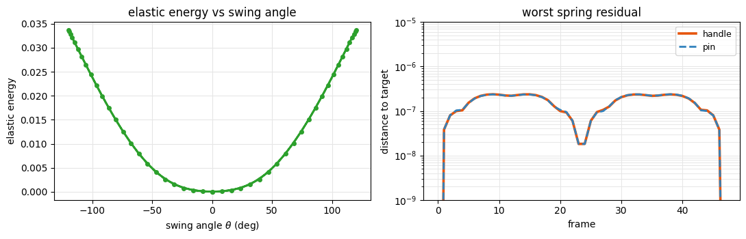
The beam’s elastic energy against the swing angle (left): zero at rest, nearly symmetric in \(\pm\theta\), and the same on the way out and back, so each pose is a well-defined minimum rather than a record of the path. Right: the worst pin and handle residuals per frame, below \(10^{-6}\) and nearly equal (they vanish at the rest frames, hence the drops at both ends), since the total forces of the two spring sets again balance.

mu_beam = np.full((len(T_beam), 1), MU)
lam_beam = np.full((len(T_beam), 1), LAM)
beam_elastic = [simkit.energies.elastic_energy(X_beam, T_beam, mu_beam, lam_beam, POSE_MATERIAL, U) for U in beam_states]
beam_residuals = {
    "handle": [np.linalg.norm(U[beam_handle] - tg, axis=1).max() for U, tg in zip(beam_states, beam_targets)],
    "pin": [np.linalg.norm(U[beam_pin] - X_beam[beam_pin], axis=1).max() for U in beam_states],
}
fig, axes = plt.subplots(1, 2, figsize=(11, 3.6))
utils.line_plot(np.rad2deg(angles), {"Neo-Hookean": beam_elastic}, xlabel=r"swing angle $\theta$ (deg)",
                ylabel="elastic energy", markers=True, ax=axes[0], title="elastic energy vs swing angle")
utils.residual_plot(beam_residuals, frames, ax=axes[1], colors={"handle": utils.HANDLE_C, "pin": utils.PIN_C},
                    xlabel="frame", ylabel="distance to target", title="worst spring residual", ylim=(1e-9, 1e-5))
fig.tight_layout()
simkit.filesystem.save_figure(fig, os.path.join(RESULTS_DIR, "beam_energy.png"),
                              copy_to=os.path.join(MEDIA_DIR, "004_beam_energy.png"))
plt.show()

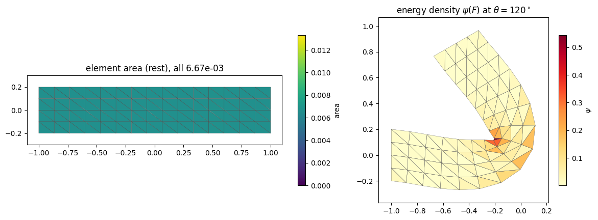
The two per-element fields behind the beam’s elastic energy \(\sum_e \text{vol}_e\,\psi(F_e)\): the element areas vol (uniform on this grid), and the energy density \(\psi(F)\) at the largest bend, drawn on the deformed beam. The energy concentrates at the inner corner of the fold, where the elements are crushed.

k = int(np.argmax(angles))
vol_beam = simkit.volume(X_beam, T_beam)
F = simkit.deformation_gradient(X_beam, T_beam, beam_states[k])
psi = simkit.energies.elastic_energy_element_F(F, mu_beam, lam_beam, POSE_MATERIAL)
fig, axes = plt.subplots(1, 2, figsize=(12, 4.2), gridspec_kw={"width_ratios": [1.5, 1]})
utils.plot_scalar_field(axes[0], X_beam, T_beam, vol_beam, vmin=0.0, vmax=2 * vol_beam.max(),
                        title=f"element area (rest), all {vol_beam.mean():.2e}", label="area")
utils.plot_scalar_field(axes[1], beam_states[k], T_beam, psi, cmap="YlOrRd",
                        title=rf"energy density $\psi(F)$ at $\theta = {np.rad2deg(angles[k]):.0f}^\circ$",
                        label=r"$\psi$")
fig.tight_layout()
simkit.filesystem.save_figure(fig, os.path.join(RESULTS_DIR, "beam_fields.png"),
                              copy_to=os.path.join(MEDIA_DIR, "004_beam_fields.png"))
plt.show()

Takeaways

• Posing = minimizing elastic energy + soft pin/handle springs, packaged as an XXX_system.

• The same setup with a different energy gives a different equilibrium.

• Soft springs leave small residuals of order \(\lVert\nabla E_{\text{elastic}}\rVert/K\).

• We solved it with Newton without looking inside. How that solve works is next.