11 · Mass Springs: from Hooke’s Law to a Sagging Cable

The spring is the simplest elastic element: two point masses joined by one edge. We derive Hooke’s law from the spring energy, give the spring a mass and compare Forward Euler, Backward Euler and BDF2 in phase space, then chain many springs into a cable and let it sag under gravity, once by minimizing its energy and once by stepping it through time.

Imports, and every tunable parameter of this notebook.

%matplotlib inline
import os
import numpy as np
import scipy as sp
import matplotlib.pyplot as plt
import simkit
from simkit.solvers import newton_solver
import utils

NOTEBOOK = "011_mass_springs"                                      # this file's name
RESULTS_DIR = utils.notebook_results_path(NOTEBOOK)                # results/011_mass_springs/
MEDIA_DIR = "media"                                                # tracked copies for the website

# 1 · single spring (node 0 is a fixed anchor, node 1 a free mass)
SPRING_L0 = 1.0               # rest length l0
K_SPRING = 1.0                # spring stiffness k (simkit's `ym`)
CURVE_L_RANGE = (0.02, 2.0)   # spring lengths for the energy / force curves
N_CURVE = 200                 # samples along those curves
SWEEP_L_RANGE = (0.1, 1.9)    # collapse / stretch range of the animation
N_SWEEP = 45                  # animation frames each way
FPS = 20                      # frame rate of the spring videos and the comparison video

# 2 · oscillator
MASS = 1.0                    # mass of the free node
U0 = 0.3                      # initial stretch u = l - l0, released from rest
DT_OSC = 0.1                  # coarse time step, so the schemes visibly differ
N_PERIODS = 3                 # simulated oscillation periods
OSC_FRAMES = 90               # frames in the oscillator video
SCHEMES = ["Forward Euler", "Backward Euler", "BDF2"]

# 3 · cable
N_NODES = 21                  # masses along the cable
CABLE_LENGTH = 4.0            # rest length of the whole cable
K_CABLE = 400.0               # stiffness k of every cable spring
RHO = 1.0                     # mass per unit rest length
GRAVITY = -9.8                # vertical acceleration
K_PIN = 1e5                   # soft-pin penalty stiffness at both ends
NEWTON_TOL = 1e-9             # step-size tolerance of the static Newton solve
NEWTON_MAX_ITERS = 50         # iteration cap of the static Newton solve
DT = 0.04                     # time step of the dynamic run
N_STEPS = 250                 # Backward-Euler steps
STEP_ITERS = 20               # Newton iterations per time step
STEP_TOL = 1e-6               # step-size tolerance of each time step's Newton solve
MONOTONE_TOL = 1e-6           # round-off allowance of the "total energy never increases" check
CABLE_FPS = 40                # frame rate of the dynamic cable video (one frame per step)
NEWTON_FPS = 2                # frame rate of the Newton-iterate video
COMPARE_FRAMES = 80           # frames in the static-vs-dynamic comparison video
FD_STEP = 1e-5                # central-difference step of the gradient check
FD_NOISE = 0.1                # size of the random state used by the gradient check
SEED = 0                      # random seed of that state
K_SWEEP = [100.0, 400.0, 1600.0]   # spring stiffnesses of the parameter study
CABLE_LIMS = ((-0.5, 4.5), (-2.6, 0.5))   # plot window of every cable figure

The notebook’s two spring networks, drawn at rest (blue squares are pinned): a single spring whose node 0 is a fixed anchor (sections 1 and 2), and a cable of N_NODES masses pinned at both ends (section 3).

X_spring = np.array([[0.0, 0.0], [SPRING_L0, 0.0]])   # node 0: anchor, node 1: free mass
E_spring = np.array([[0, 1]])
anchor = X_spring[:1]

X = np.column_stack([np.linspace(0.0, CABLE_LENGTH, N_NODES), np.zeros(N_NODES)])
E = np.column_stack([np.arange(N_NODES - 1), np.arange(1, N_NODES)])   # spring e joins nodes e, e+1
pin_idx = np.array([0, N_NODES - 1])
n, dim = X.shape

fig, (ax_s, ax_c) = plt.subplots(1, 2, figsize=(12, 2.4), gridspec_kw={"width_ratios": [1, 2.4]})
utils.plot_spring_network(ax_s, X_spring, E_spring, pins=[0], node_size=50, lw=3,
                          title="single spring", lims=((-0.25, 1.35), (-0.3, 0.3)))
utils.plot_spring_network(ax_c, X, E, pins=pin_idx, node_size=50, lw=3,
                          title=f"cable: {N_NODES} masses, {len(E)} springs",
                          lims=((-0.25, CABLE_LENGTH + 0.25), (-0.3, 0.3)))
fig.tight_layout()
simkit.filesystem.save_figure(fig, os.path.join(RESULTS_DIR, "meshes.png"),
                              copy_to=os.path.join(MEDIA_DIR, "011_meshes.png"))
plt.show()

1 · The elastic energy of a single spring (Hooke’s law)

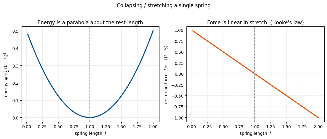
A spring stores energy through its edge vector \(d = x_j - x_i\) (blind to translation), its length \(l = \lVert d\rVert\) (blind to rotation) and its stretch \(l - l_0\). Differentiating the quadratic energy gives the force, linear in the stretch and pointing back to rest: Hooke’s law is derived, not assumed.

\[ \psi = \tfrac12\,k\,(l-l_0)^2, \qquad f = -\frac{d\psi}{dl} = -k\,(l-l_0). \]

anchored_spring_system turns that one spring into a mechanical system in the free mass’s position \(x \in \mathbb{R}^2\); the anchor is not a degree of freedom. It builds \(\psi\) and its derivatives from simkit’s per-edge mass_springs_*_element_d, whose ym is the stiffness \(k\) itself (no rest-length normalization). Sections 1 and 2 hand its three functions to plots, integrators and Newton.

def anchored_spring_system(anchor, k, l0):
    """One spring from a fixed `anchor` to a free mass at x (2 DOFs): psi = 1/2 k (|x - anchor| - l0)^2."""
    ym = np.array([[k]])
    rest_length = np.array([[l0]])

    def energy_func(x):
        d = x.reshape(1, 2) - anchor                                   # edge vector
        E_spring = simkit.energies.mass_springs_energy_element_d(d, ym, rest_length).item()
        E_total = E_spring
        return E_total

    def gradient_func(x):
        d = x.reshape(1, 2) - anchor
        g_spring = simkit.energies.mass_springs_gradient_element_d(d, ym, rest_length).reshape(-1, 1)
        g_total = g_spring
        return g_total

    def hessian_func(x):
        d = x.reshape(1, 2) - anchor
        H_spring = simkit.energies.mass_springs_hessian_element_d(d, ym, rest_length)[0]
        H_total = H_spring
        return H_total

    return energy_func, gradient_func, hessian_func

Slide the free mass along the axis from nearly collapsed to twice the rest length, reading the energy from energy_func and the force from -gradient_func. The printed deviations from the closed forms above are round-off; the plots show a parabola about \(l_0\) and a straight force line crossing zero at \(l_0\).

energy_func, gradient_func, hessian_func = anchored_spring_system(anchor, K_SPRING, SPRING_L0)

lengths = np.linspace(*CURVE_L_RANGE, N_CURVE)
psi, force = [], []
for l in lengths:
    x = np.array([[l], [0.0]])
    psi.append(energy_func(x))
    force.append(-gradient_func(x)[0, 0])                 # axial force on the free mass
psi, force = np.array(psi), np.array(force)
print(f"max |psi - k(l-l0)^2/2| = {np.abs(psi - 0.5 * K_SPRING * (lengths - SPRING_L0) ** 2).max():.1e},  "
      f"max |f + k(l-l0)| = {np.abs(force + K_SPRING * (lengths - SPRING_L0)).max():.1e}")

fig, (ax_e, ax_f) = plt.subplots(1, 2, figsize=(11, 4.5))
ax_e.plot(lengths, psi, color=utils.SPRING_EDGE, lw=2.5)
ax_e.axvline(SPRING_L0, color="0.6", ls="--", lw=1.5)
ax_e.set_xlabel("spring length  $l$")
ax_e.set_ylabel(r"energy  $\psi=\frac{1}{2}k(l-l_0)^2$")
ax_e.set_title("Energy is a parabola about the rest length")
ax_e.grid(True, color="0.92")
ax_f.plot(lengths, force, color=utils.SPRING_NODE, lw=2.5)
ax_f.axhline(0, color="0.6", lw=1.0)
ax_f.axvline(SPRING_L0, color="0.6", ls="--", lw=1.5)
ax_f.set_xlabel("spring length  $l$")
ax_f.set_ylabel(r"restoring force  $f=-k(l-l_0)$")
ax_f.set_title("Force is linear in stretch  (Hooke's law)")
ax_f.grid(True, color="0.92")
fig.suptitle("Collapsing / stretching a single spring", y=1.02)
fig.tight_layout()
simkit.filesystem.save_figure(fig, os.path.join(RESULTS_DIR, "hooke.png"),
                              copy_to=os.path.join(MEDIA_DIR, "011_hooke.png"))
plt.show()

max |psi - k(l-l0)^2/2| = 0.0e+00,  max |f + k(l-l0)| = 1.1e-16

Now collapse and re-stretch the spring while tracing its energy in lock-step, so the quadratic well around \(l_0\) is unmistakable (the gray dashes are the rest shape).

sweep = np.concatenate([np.linspace(*SWEEP_L_RANGE, N_SWEEP), np.linspace(*SWEEP_L_RANGE[::-1], N_SWEEP)])
states, psi_sweep = [], []
for l in sweep:
    x = np.array([[l], [0.0]])
    states.append(np.vstack([anchor, x.T]))
    psi_sweep.append(energy_func(x))

fig, anim = utils.animate_springs_energy(
    states, E_spring, sweep, {"elastic": psi_sweep}, rest=X_spring, lims=((-0.4, 2.2), (-0.8, 0.8)),
    xlabel="spring length  $l$", ylabel="elastic energy", scene_title="spring (gray = rest)",
    title="energy vs length", colors={"elastic": utils.SPRING_EDGE}, pin_pts=anchor)
video = simkit.filesystem.save_animation(anim, os.path.join(RESULTS_DIR, "spring_collapse.mp4"), fps=FPS,
                                         copy_to=os.path.join(MEDIA_DIR, "011_spring_collapse.mp4"))
plt.close(fig)
utils.embed_video(video)

2 · Adding inertia: integrators and the phase portrait

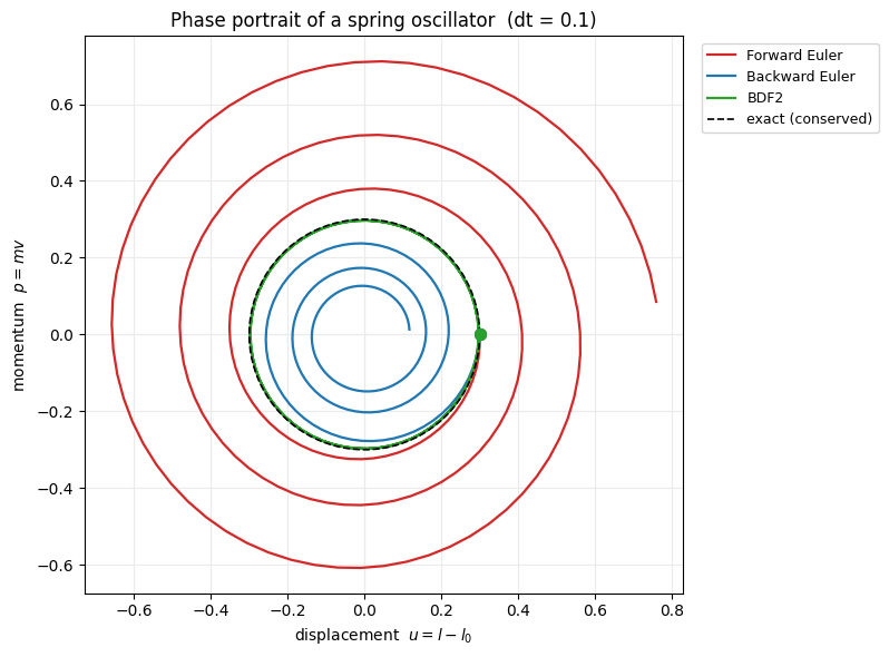
Give the free node a mass \(m\) and release it from rest at stretch \(u_0\). Along the axis, with \(u = l - l_0\), Newton’s second law is a harmonic oscillator, \(m\ddot u = -k u\) with \(\omega = \sqrt{k/m}\). The exact motion conserves \(H = \tfrac12 k u^2 + \tfrac12 m v^2\), so in the displacement–momentum plane \((u,\,p = mv)\) it traces a closed ellipse forever; a good integrator keeps that loop closed.

simulate marches one of simkit’s integrators, all fed the same anchored_spring_system: forward_euler only reads the force \(-\nabla\psi\), while backward_euler and bdf2 minimize \(\psi\) plus an inertia term with Newton (one Newton step is exact here, because \(\psi\) is quadratic along the axis). Velocities come from the schemes’ own difference formulas, and the total energy \(H\) is recorded at every step. The print gives \(\omega\), the period and the number of steps covering N_PERIODS periods.

M_osc = MASS * sp.sparse.eye(2).tocsc()          # point mass on the free node's two DOFs
omega = np.sqrt(K_SPRING / MASS)
period = 2 * np.pi / omega
n_osc = int(round(N_PERIODS * period / DT_OSC))

def simulate(scheme):
    """Release the free mass from rest at stretch U0 and march `scheme`; return u, v and H per step."""
    x0 = np.array([[SPRING_L0 + U0], [0.0]])
    hist = [x0, x0, x0, x0]                        # position history, newest last: at rest for t <= 0
    v = np.zeros((2, 1))
    vs = [v]
    for _ in range(n_osc):
        if scheme == "Forward Euler":
            x, v = simkit.integrators.forward_euler(hist[-1], v, gradient_func, M_osc, DT_OSC)
        elif scheme == "Backward Euler":
            x = simkit.integrators.backward_euler(hist[-1], hist[-2], energy_func, gradient_func,
                                                  hessian_func, M_osc, DT_OSC)
            v = simkit.energies.velocity_be(x, hist[-1], DT_OSC)
        else:
            x = simkit.integrators.bdf2(hist[-1], hist[-2], hist[-3], hist[-4], energy_func, gradient_func,
                                        hessian_func, M_osc, DT_OSC)
            v = simkit.energies.velocity_bdf2(x, hist[-1], hist[-2], DT_OSC)
        hist.append(x)
        vs.append(v)
    xs = hist[3:]
    u = np.array([x[0, 0] for x in xs]) - SPRING_L0
    vel = np.array([v[0, 0] for v in vs])
    H_spring = np.array([energy_func(x) for x in xs])
    H_kinetic = 0.5 * MASS * vel ** 2
    H_total = H_spring + H_kinetic
    return {"u": u, "v": vel, "H": H_total}

traj = {}
for s in SCHEMES:
    traj[s] = simulate(s)
print(f"omega = {omega:.3f},  period = {period:.3f},  {n_osc} steps of dt = {DT_OSC}")

omega = 1.000,  period = 6.283,  188 steps of dt = 0.1

Why they differ: on the state \(y = [u, v]\) each scheme is a linear map of \(y' = Ay\), with \(A = \begin{pmatrix}0 & 1\\ -k/m & 0\end{pmatrix}\). The cell builds the maps and prints each one’s per-step amplification (largest eigenvalue magnitude: above 1 grows, below 1 damps). It also confirms that simkit’s trajectories are exactly these maps, to round-off.

scheme	one step	phase-space behaviour
Forward Euler	\(y_{n+1} = (I + hA)\,y_n\)	spirals outward (gains energy)
Backward Euler	\((I - hA)\,y_{n+1} = y_n\)	spirals inward (numerical damping)
BDF2	\((3I - 2hA)\,y_{n+1} = 4y_n - y_{n-1}\)	nearly closed (2nd order)

A = np.array([[0.0, 1.0], [-K_SPRING / MASS, 0.0]])
I2 = np.eye(2)
B = np.linalg.inv(3 * I2 - 2 * DT_OSC * A)
step_maps = {
    "Forward Euler": I2 + DT_OSC * A,
    "Backward Euler": np.linalg.inv(I2 - DT_OSC * A),
    "BDF2": np.block([[4 * B, -B], [I2, np.zeros((2, 2))]]),     # acts on [y_n; y_{n-1}]
}
for s, G in step_maps.items():
    z = np.tile([U0, 0.0], G.shape[0] // 2)                      # at rest before release
    Y = [z[:2]]
    for _ in range(n_osc):
        z = G @ z
        Y.append(z[:2])
    deviation = np.abs(np.array(Y) - np.column_stack([traj[s]["u"], traj[s]["v"]])).max()
    print(f"{s:15s} per-step amplification = {np.abs(np.linalg.eigvals(G)).max():.5f},  "
          f"max |simkit - map| = {deviation:.1e}")

Forward Euler   per-step amplification = 1.00499,  max |simkit - map| = 3.3e-16
Backward Euler  per-step amplification = 0.99504,  max |simkit - map| = 8.5e-15
BDF2            per-step amplification = 0.99998,  max |simkit - map| = 5.0e-14

The phase portrait

Displacement against momentum: Forward Euler spirals out, Backward Euler spirals in, and BDF2 sits on the exact, energy-conserving ellipse (dashed).

fig, ax = utils.phase_plot({s: np.column_stack([traj[s]["u"], MASS * traj[s]["v"]]) for s in SCHEMES},
                           xlabel="displacement  $u = l - l_0$", ylabel="momentum  $p = m v$",
                           title=f"Phase portrait of a spring oscillator  (dt = {DT_OSC})",
                           figsize=(8.4, 6))
theta = np.linspace(0, 2 * np.pi, 200)
ax.plot(U0 * np.cos(theta), MASS * omega * U0 * np.sin(theta), "k--", lw=1.2, label="exact (conserved)")
ax.set_aspect("equal")
ax.legend(loc="upper left", bbox_to_anchor=(1.02, 1), fontsize=9)    # beside the axes, off the spirals
fig.tight_layout()
simkit.filesystem.save_figure(fig, os.path.join(RESULTS_DIR, "phase_portrait.png"),
                              copy_to=os.path.join(MEDIA_DIR, "011_phase_portrait.png"))
plt.show()

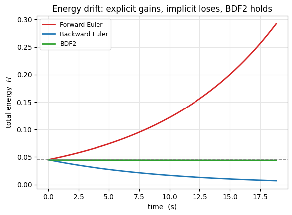
The same story as a time series of the total energy \(H\), which every scheme should hold at its initial value \(\tfrac12 k u_0^2\) (dashed): explicit gains, implicit loses, BDF2 holds.

t_osc = np.arange(n_osc + 1) * DT_OSC
fig, ax = utils.line_plot(t_osc, {s: traj[s]["H"] for s in SCHEMES}, xlabel="time  (s)",
                          ylabel="total energy  $H$", colors=utils.INTEGRATOR_COLORS,
                          title="Energy drift: explicit gains, implicit loses, BDF2 holds")
ax.axhline(0.5 * K_SPRING * U0 ** 2, color="0.5", ls="--", lw=1.2)
simkit.filesystem.save_figure(fig, os.path.join(RESULTS_DIR, "energy_drift.png"),
                              copy_to=os.path.join(MEDIA_DIR, "011_energy_drift.png"))
plt.show()

And the three integrators as actual oscillating springs, side by side: the explicit one’s swing grows, the implicit one’s shrinks, BDF2’s stays steady.

stride = max(1, (n_osc + 1) // OSC_FRAMES)
panels = []
for s in SCHEMES:
    states = [np.vstack([anchor, [[SPRING_L0 + u, 0.0]]]) for u in traj[s]["u"][::stride]]
    panels.append({"states": states, "E": E_spring, "title": s})

fig, anim = utils.animate_springs_grid(
    panels, lims=((-0.3, 2.0), (-0.4, 0.4)), fps=FPS, pin_pts=anchor, figsize=(13, 2.6),
    suptitle="Same spring, same dt: explicit grows, implicit shrinks, BDF2 steady")
fig.tight_layout()
video = simkit.filesystem.save_animation(anim, os.path.join(RESULTS_DIR, "oscillators.mp4"), fps=FPS,
                                         copy_to=os.path.join(MEDIA_DIR, "011_oscillators.mp4"))
plt.close(fig)
utils.embed_video(video)

3 · A cable: many springs glued together

One spring resists only stretch. Chain many end to end and pin both ends, and the assembly behaves like an elastic cable: under gravity the interior masses drop until spring tension balances weight (an elastic catenary). Springs carry no bending stiffness, so this is a cable, not a beam; bending is the next ingredient. In stacked positions \(x\) the cable’s potential \(\Phi\), and the objective of one Backward-Euler step, are

\[ \Phi(x) = \underbrace{\textstyle\sum_e \tfrac12 k\,(l_e-l_{0,e})^2}_{\text{springs}} + \underbrace{\tfrac12 x^\top Q x + b^\top x}_{\text{pins}} - \underbrace{f_g^\top x}_{\text{gravity}}, \qquad \Phi(x) + \underbrace{\tfrac{1}{2h^2}\lVert x - \tilde x\rVert_M^2}_{\text{inertia}},\quad \tilde x = 2x_n - x_{n-1}. \]

The cable’s constant operators, built once from simkit: the stacked edge-vector operator \(J\) (\(d = Jx\)), the rest lengths \(l_0\), the lumped mass matrix \(M\), the gravity force \(f_g\) and the soft-pin penalty \((Q, b)\) from dirichlet_penalty. The print checks that the lumped masses add up to \(\rho L\) and the weights to \(\rho L g\).

J = sp.sparse.kron(simkit.edge_displacement_jacobian(X, E), sp.sparse.eye(dim)).tocsc()   # d = J x
l0 = simkit.edge_lengths(X, E).reshape(-1, 1)                        # rest length of every spring
vol = np.ones((len(E), 1))                                           # unit weight per spring
M_nodes = simkit.massmatrix(X, E, rho=RHO)                           # lumped mass of every node
M = sp.sparse.kron(M_nodes, sp.sparse.eye(dim)).tocsc()              # the same mass on every DOF
f_g = simkit.gravity_force(X, E, a=GRAVITY, rho=RHO).reshape(-1, 1)  # weight of every node
Q_pin, b_pin = simkit.dirichlet_penalty(pin_idx, X[pin_idx], n, K_PIN)   # soft pins at both ends
print(f"J: {J.shape},  total mass = {M_nodes.sum():.3f} (rho L = {RHO * CABLE_LENGTH:.3f}),  "
      f"total weight = {f_g.sum():.3f} (rho L g = {RHO * CABLE_LENGTH * GRAVITY:.3f})")

J: (40, 42),  total mass = 4.000 (rho L = 4.000),  total weight = -39.200 (rho L g = -39.200)

cable_system closes over those operators and builds every term from simkit, one per line: the springs with mass_springs_*_z on \(d = Jx\), the pins as a quadratic, and gravity as a linear term. Called without a previous state it is the quasi-static potential \(\Phi\); given \((x_n, x_{n-1})\) it adds the Backward-Euler inertia term (kinetic_*_be), so one function drives both runs.

def cable_system(k, x_curr=None, x_prev=None, h=DT):
    """Cable potential (springs + pins + gravity) with spring stiffness k, in stacked positions x.

    Closes over the constant operators J, l0, vol, M, f_g, Q_pin, b_pin built above.
    Pass x_curr, x_prev to add the Backward-Euler inertia term."""
    ym = np.full((len(E), 1), k)
    dynamic = x_curr is not None

    def energy_func(x):
        E_spring = simkit.energies.mass_springs_energy_z(x, J, ym, vol, l0)
        E_pin = simkit.energies.quadratic_energy(x, Q_pin, b_pin)
        E_gravity = -(f_g.T @ x).item()
        E_inertia = simkit.energies.kinetic_energy_be(x, x_curr, x_prev, M, h) if dynamic else 0.0
        E_total = E_spring + E_pin + E_gravity + E_inertia
        return E_total

    def gradient_func(x):
        g_spring = simkit.energies.mass_springs_gradient_z(x, J, ym, vol, l0)
        g_pin = simkit.energies.quadratic_gradient(x, Q_pin, b_pin)
        g_gravity = -f_g
        g_inertia = simkit.energies.kinetic_gradient_be(x, x_curr, x_prev, M, h) if dynamic else 0.0
        g_total = g_spring + g_pin + g_gravity + g_inertia
        return g_total

    def hessian_func(x):
        H_spring = simkit.energies.mass_springs_hessian_z(x, J, ym, vol, l0, psd=True)
        H_pin = simkit.energies.quadratic_hessian(Q_pin)
        H_inertia = simkit.energies.kinetic_hessian_be(M, h) if dynamic else 0.0 * M
        H_total = H_spring + H_pin + H_inertia                   # gravity is linear: no Hessian term
        return H_total

    return energy_func, gradient_func, hessian_func

Before trusting Newton with it, check the gradient of the full dynamic system (all four terms) against central differences of its energy (simkit.gradient_cfd) at a random stretched state. The relative error should be tiny.

x_rest = X.reshape(-1, 1).copy()
rng = np.random.default_rng(SEED)
noise = FD_NOISE * rng.standard_normal((n, dim))
noise[pin_idx] = 0.0                                             # keep the pins on target
x_test = (X + noise).reshape(-1, 1)

step_energy, step_gradient, _ = cable_system(K_CABLE, x_curr=x_rest, x_prev=x_rest)
g_fd = simkit.gradient_cfd(lambda y: np.array(step_energy(y.reshape(-1, 1))), x_test.ravel(), FD_STEP)
g = step_gradient(x_test)
print(f"relative gradient error vs central differences: {np.linalg.norm(g - g_fd.reshape(-1, 1)) / np.linalg.norm(g):.1e}")

relative gradient error vs central differences: 6.7e-08

Without inertia: static equilibrium via Newton

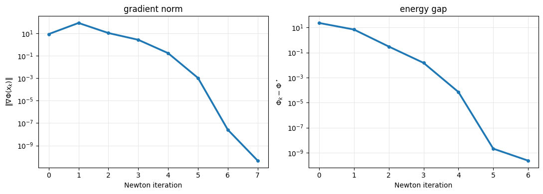
No time, no velocity: minimize \(\Phi\) from the flat chain, one Newton step at a time, recording every iterate until the step is below NEWTON_TOL. The chain drops into its sag within a few iterations while the energy gap \(\Phi_k - \Phi^\star\) collapses to zero.

phi_energy, phi_gradient, phi_hessian = cable_system(K_CABLE)

x = x_rest.copy()
static_states, phi_hist, grad_hist = [X.copy()], [phi_energy(x)], [np.linalg.norm(phi_gradient(x))]
for _ in range(NEWTON_MAX_ITERS):
    x_next = newton_solver(x, phi_energy, phi_gradient, phi_hessian, max_iter=1)
    step = np.linalg.norm(x_next - x)
    x = x_next
    static_states.append(x.reshape(n, dim).copy())
    phi_hist.append(phi_energy(x))
    grad_hist.append(np.linalg.norm(phi_gradient(x)))
    if step < NEWTON_TOL:
        break
x_static = x.copy()
phi_star = phi_hist[-1]
energy_gap = np.array(phi_hist) - phi_star
print(f"static: {len(static_states) - 1} Newton iterations,  |grad| = {grad_hist[-1]:.1e},  "
      f"max sag = {-x_static.reshape(n, dim)[:, 1].min():.3f}")

fig, anim = utils.animate_springs_energy(
    static_states, E, np.arange(len(static_states)), {"potential": energy_gap}, rest=X, lims=CABLE_LIMS,
    xlabel="Newton iteration", ylabel=r"energy gap  $\Phi_k - \Phi^\star$", scene_title="static sag (gray = rest)",
    title="energy minimized", colors={"potential": utils.ENERGY_COLORS["potential"]}, pin_pts=X[pin_idx])
video = simkit.filesystem.save_animation(anim, os.path.join(RESULTS_DIR, "cable_static.mp4"), fps=NEWTON_FPS,
                                         copy_to=os.path.join(MEDIA_DIR, "011_cable_static.mp4"))
plt.close(fig)
utils.embed_video(video)

static: 7 Newton iterations,  |grad| = 4.5e-11,  max sag = 1.258

The same solve on a log scale. The first step overshoots the sag (the line search only asks for lower energy), so the gradient norm briefly rises; after that both curves fall ever faster, the last steps quadratically, down to round-off.

fig, (ax_g, ax_e) = plt.subplots(1, 2, figsize=(11, 4))
utils.residual_plot({"Newton": grad_hist}, ax=ax_g, markers=True, xlabel="Newton iteration",
                    ylabel=r"$\|\nabla\Phi(x_k)\|$", title="gradient norm")
utils.residual_plot({"Newton": energy_gap}, ax=ax_e, markers=True, xlabel="Newton iteration",
                    ylabel=r"$\Phi_k - \Phi^\star$", title="energy gap")
fig.tight_layout()
simkit.filesystem.save_figure(fig, os.path.join(RESULTS_DIR, "newton_convergence.png"),
                              copy_to=os.path.join(MEDIA_DIR, "011_newton_convergence.png"))
plt.show()

Two scalar fields of the cable: the lumped mass of each node (the two end nodes own half a spring each, so they get half the mass), and the tension \(k\,(l_e - l_{0,e})\) of each spring at the static equilibrium. The tension is largest next to the pins, which carry the whole weight, and smallest at the bottom.

m_nodes = M_nodes.diagonal()
X_static = x_static.reshape(n, dim)
tension = K_CABLE * (simkit.edge_lengths(X_static, E) - l0.ravel())

fig, (ax_m, ax_t) = plt.subplots(2, 1, figsize=(8, 6.6), gridspec_kw={"height_ratios": [1, 2.6]})
utils.plot_spring_network(ax_m, X, E, node_values=m_nodes, node_size=70, cmap="viridis",
                          title="lumped node mass (at rest)", label="mass", vmin=0.0,
                          lims=(CABLE_LIMS[0], (-0.5, 0.5)))
utils.plot_spring_network(ax_t, X_static, E, edge_values=tension, pins=pin_idx, node_size=20, lw=3,
                          cmap="plasma", title="spring tension at equilibrium", label=r"$k(l-l_0)$",
                          lims=CABLE_LIMS)
fig.tight_layout()
simkit.filesystem.save_figure(fig, os.path.join(RESULTS_DIR, "cable_fields.png"),
                              copy_to=os.path.join(MEDIA_DIR, "011_cable_fields.png"))
plt.show()
print(f"tension: {tension.min():.1f} at the bottom  ->  {tension.max():.1f} next to the pins")

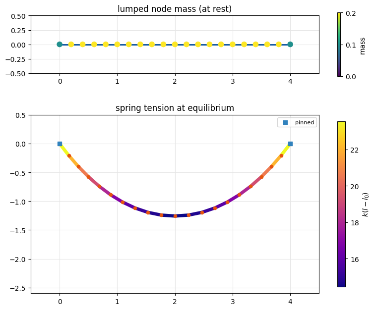
tension: 14.4 at the bottom  ->  23.5 next to the pins

With inertia: Backward-Euler dynamics from rest

Release the flat chain and march it N_STEPS steps: each step rebuilds cable_system with the last two states and minimizes it with Newton, starting from the inertial guess \(\tilde x\). The chain falls, overshoots and oscillates, and Backward Euler’s numerical damping rings the kinetic energy down.

x_curr, x_prev = x_rest.copy(), x_rest.copy()                    # released from rest
dyn_states = [X.copy()]
ke_hist = [0.0]                                                  # kinetic energy
dist_hist = [np.linalg.norm((x_rest - x_static).reshape(n, dim), axis=1).max()]   # largest node distance to x*
total_hist = [phi_hist[0] - phi_star]                            # kinetic + potential above the minimum
for _ in range(N_STEPS):
    step_energy, step_gradient, step_hessian = cable_system(K_CABLE, x_curr=x_curr, x_prev=x_prev)
    x_tilde = simkit.energies.be_target(x_curr, x_prev, DT)
    x_next = newton_solver(x_tilde, step_energy, step_gradient, step_hessian, max_iter=STEP_ITERS,
                           tolerance=STEP_TOL)
    x_prev, x_curr = x_curr, x_next
    v = simkit.energies.velocity_be(x_curr, x_prev, DT)
    ke = 0.5 * (v.T @ M @ v).item()                              # kinetic energy
    pe = phi_energy(x_curr) - phi_star                           # potential above the minimum
    total = ke + pe
    dyn_states.append(x_curr.reshape(n, dim).copy())
    ke_hist.append(ke)
    dist_hist.append(np.linalg.norm((x_curr - x_static).reshape(n, dim), axis=1).max())
    total_hist.append(total)
t_hist = np.arange(N_STEPS + 1) * DT
print(f"dynamic: max sag during the run = {max(-s[:, 1].min() for s in dyn_states):.3f},  "
      f"final max sag = {-x_curr.reshape(n, dim)[:, 1].min():.3f} (static {-X_static[:, 1].min():.3f}),  "
      f"final KE = {ke_hist[-1]:.1e}")

fig, anim = utils.animate_springs_energy(
    dyn_states, E, t_hist, {"kinetic": ke_hist}, rest=X,
    lims=CABLE_LIMS, xlabel="time  (s)", ylabel="kinetic energy", scene_title="dynamic sag (Backward Euler)",
    title="kinetic energy rings down", colors={"kinetic": utils.ENERGY_COLORS["kinetic"]}, pin_pts=X[pin_idx])
video = simkit.filesystem.save_animation(anim, os.path.join(RESULTS_DIR, "cable_dynamic.mp4"), fps=CABLE_FPS,
                                         copy_to=os.path.join(MEDIA_DIR, "011_cable_dynamic.mp4"))
plt.close(fig)
utils.embed_video(video)

dynamic: max sag during the run = 1.981,  final max sag = 1.268 (static 1.258),  final KE = 1.7e-04

Same equilibrium, two roads

Quasi-static minimization (each Newton iterate held for a few frames) and full dynamics, side by side: both settle to the same sagged shape.

static_frames = [static_states[min(i * len(static_states) // COMPARE_FRAMES, len(static_states) - 1)]
                 for i in range(COMPARE_FRAMES)]
dynamic_frames = [dyn_states[i] for i in np.linspace(0, N_STEPS, COMPARE_FRAMES).astype(int)]

fig, anim = utils.animate_springs_grid(
    [{"states": static_frames, "E": E, "title": "without inertia (Newton iterates)"},
     {"states": dynamic_frames, "E": E, "title": "with inertia (Backward Euler)"}],
    lims=CABLE_LIMS, fps=FPS, pin_pts=X[pin_idx], figsize=(11, 3.8),
    suptitle="Cable sag: minimization vs dynamics settle to the same shape")
video = simkit.filesystem.save_animation(anim, os.path.join(RESULTS_DIR, "cable_compare.mp4"), fps=FPS,
                                         copy_to=os.path.join(MEDIA_DIR, "011_cable_compare.mp4"))
plt.close(fig)
utils.embed_video(video)

Quantitatively: the largest vertex distance between the dynamic cable and the static equilibrium, and the total energy above the static minimum, \(\tfrac12 v^\top M v + \Phi(x) - \Phi^\star\). Both decay toward zero, and the total energy never increases: Backward Euler only removes energy.

fig, (ax_d, ax_h) = plt.subplots(1, 2, figsize=(11, 4))
utils.residual_plot({"dynamic": dist_hist}, t_hist, ax=ax_d, xlabel="time  (s)",
                    ylabel=r"$\max_i \|x_i(t) - x_i^\star\|$", title="distance to the static shape")
utils.residual_plot({"dynamic": total_hist}, t_hist, ax=ax_h, xlabel="time  (s)",
                    ylabel=r"$\frac{1}{2}v^\top M v + \Phi - \Phi^\star$", title="total energy above the minimum")
fig.tight_layout()
simkit.filesystem.save_figure(fig, os.path.join(RESULTS_DIR, "cable_settling.png"),
                              copy_to=os.path.join(MEDIA_DIR, "011_cable_settling.png"))
plt.show()
print(f"total energy monotone (up to round-off): {bool(np.all(np.diff(total_hist) <= MONOTONE_TOL))},  "
      f"final distance = {dist_hist[-1]:.1e}")

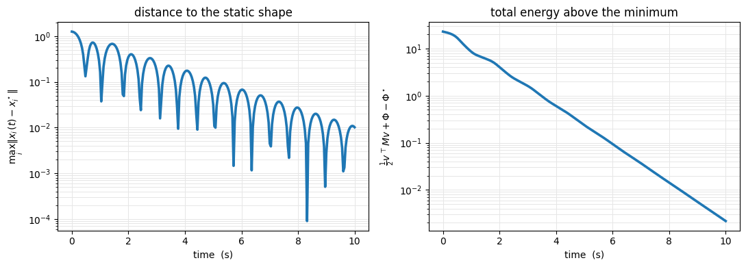
total energy monotone (up to round-off): True,  final distance = 1.0e-02

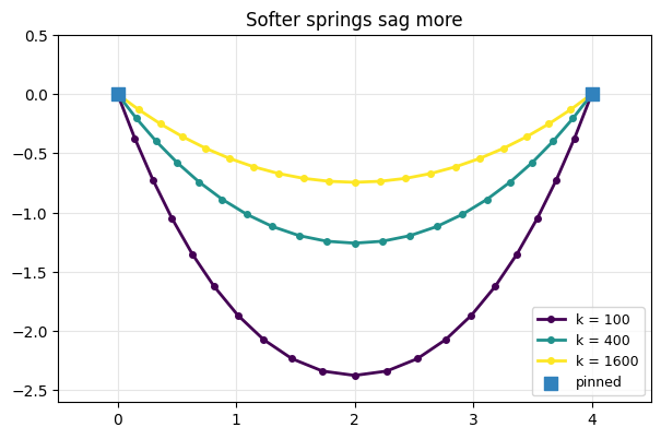
Finally, a quick parameter study: re-solve the static sag for each stiffness in K_SWEEP. Softer springs stretch more and sag deeper.

sags = {}
for k in K_SWEEP:
    energy_k, gradient_k, hessian_k = cable_system(k)
    x_k = newton_solver(x_rest.copy(), energy_k, gradient_k, hessian_k, max_iter=NEWTON_MAX_ITERS, tolerance=NEWTON_TOL)
    sags[k] = x_k.reshape(n, dim)
    print(f"k = {k:6g}:  max sag = {-sags[k][:, 1].min():.3f}")

fig, ax = plt.subplots(figsize=(7, 4.5))
utils.setup_axes(ax, *CABLE_LIMS, title="Softer springs sag more")
cmap = plt.get_cmap("viridis")
for j, (k, X_k) in enumerate(sags.items()):
    ax.plot(X_k[:, 0], X_k[:, 1], "-o", ms=4, lw=2, color=cmap(j / max(1, len(sags) - 1)), label=f"k = {k:g}")
ax.scatter(X[pin_idx, 0], X[pin_idx, 1], s=70, marker="s", color=utils.PIN_C, zorder=5, label="pinned")
ax.legend(fontsize=9, loc="lower right")
simkit.filesystem.save_figure(fig, os.path.join(RESULTS_DIR, "cable_stiffness.png"),
                              copy_to=os.path.join(MEDIA_DIR, "011_cable_stiffness.png"))
plt.show()

k =    100:  max sag = 2.374
k =    400:  max sag = 1.258
k =   1600:  max sag = 0.744

Takeaways

• A spring stores \(\tfrac12 k (l-l_0)^2\); differentiating gives the linear Hooke force \(-k(l-l_0)\).

• With inertia the integrator decides the energy behaviour: Forward Euler gains it (unstable), Backward Euler bleeds it (damped), BDF2 nearly conserves it, vivid in the phase portrait.

• Many springs make an elastic cable; gravity sags it into an elastic catenary, and the quasi-static minimization and the dynamic Backward-Euler run settle to the same equilibrium.