12 · Quadratic (P2) finite elements

Every element so far has been linear (P1): positions vary linearly inside a triangle, so the deformation gradient \(F\) is constant per element. Quadratic (P2) elements add a node at every edge midpoint, so positions vary quadratically, \(F\) varies within each element, and bending is captured far more accurately on the same mesh. We plot both bases, sag a coarse cantilever with each, show why P2 is not just a subdivided mesh, and measure convergence rates with a manufactured solution.

Imports, and every tunable parameter of this notebook.

%matplotlib inline
import os
import numpy as np
import scipy as sp
import matplotlib.pyplot as plt
from matplotlib.colors import LogNorm
import igl
import simkit
import utils

NOTEBOOK = "012_p2_finite_elements"                               # this file's name
RESULTS_DIR = utils.notebook_results_path(NOTEBOOK)               # results/012_p2_finite_elements/
MEDIA_DIR = "media"                                               # tracked copies for the website
# Part A: basis functions
BASIS_SUBDIVS = 5                      # upsampling levels of the reference triangle (4^k samples)
# Part B: cantilever beam, left edge pinned, sagging under gravity
BEAM_NX, BEAM_NY = 5, 4                # grid vertices (deliberately coarse)
BEAM_WIDTH, BEAM_HEIGHT = 2.0, 0.3     # beam size
MATERIAL = "macklin-mueller-neo-hookean"  # hyperelastic model of the beam (simkit material name)
YM, PR = 300.0, 0.4                    # Young's modulus, Poisson ratio
RHO = 1.0                              # density
GRAVITY = -9.8                         # vertical acceleration
K_PIN = 1e7                            # soft-pin stiffness
QUAD_ORDER = 2                         # P2 cubature order for the elastic energy
DT = 0.01                              # backward-Euler timestep
T_TOTAL = 1.2                          # simulated time
N_FRAMES = 48                          # frames sampled for the animation
FPS = 24                               # animation frame rate
STATIC_FPS = 2                         # frame rate of the rest -> equilibrium clip
STEP_ITERS, STEP_TOL = 30, 1e-8        # Newton iterations / tolerance per timestep
STATIC_ITERS, STATIC_TOL = 200, 1e-9   # Newton iterations / tolerance for static equilibrium
FD_STEP = 1e-6                         # central-difference step for the gradient check
FD_NOISE = 0.05                        # random perturbation of the check state
SEED = 0                               # random seed for the gradient check
EDGE_SAMPLES = 12                      # samples per curved P2 edge when drawing
# Subdivision demo
BEND = 0.5                             # bending field phi(x, y) = (x, y + BEND x^2)
DEMO_CORNERS = np.array([[-1.0, 0.0], [1.0, 0.0], [0.0, 1.2]])  # triangle bent by phi
TRUTH_SAMPLES = 160                    # samples per edge of the exact bent outline
# Part C: manufactured-solution convergence (linear elasticity on the unit square)
MMS_YM, MMS_PR = 1.0, 0.3              # Young's modulus, Poisson ratio
MMS_RESOLUTIONS = [4, 8, 16, 32]       # elements per side of the unit square
MMS_STIFF_QUAD_ORDER = 2               # P2 stiffness cubature (exact for linear elasticity)
MMS_QUAD_ORDER = 4                     # quadrature order for the load and error integrals
MMS_K_PIN = 1e10                       # boundary pin stiffness (u = 0)
MMS_SHOW_RES = 8                       # resolution whose pointwise error field is plotted
# plotting
COLORS = {"P1": "#d62728", "P2": "#1f77b4"}

Part A — The basis functions

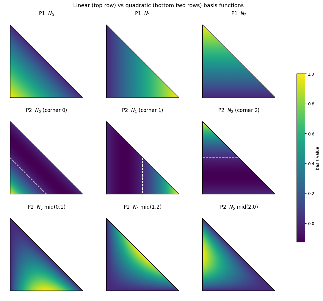
On the reference triangle the P1 hats are the barycentric coordinates \(L_i\) (planar ramps). The P2 corner functions \(N_i = L_i(2L_i - 1)\) curve and dip slightly negative (down to \(-\tfrac18\)) in the band between the dashed line \(L_i = \tfrac12\) and the opposite edge, and the midpoint functions \(N = 4L_aL_b\) are bumps centred on their edge. simkit.p2_shape_functions evaluates them; each panel is a scalar field on an upsampled reference triangle.

ref_V, ref_T = igl.upsample(np.array([[0.0, 0.0], [1.0, 0.0], [0.0, 1.0]]), np.array([[0, 1, 2]]), BASIS_SUBDIVS)
L = np.column_stack([1.0 - ref_V.sum(axis=1), ref_V])                # barycentric coordinates of every sample
P1_basis = L                                                          # (npts, 3)
P2_basis = np.array([simkit.p2_shape_functions(Li, 3)[0] for Li in L])  # (npts, 6), corners then midpoints

titles = [r"P1  $N_0$", r"P1  $N_1$", r"P1  $N_2$",
          r"P2  $N_0$ (corner 0)", r"P2  $N_1$ (corner 1)", r"P2  $N_2$ (corner 2)",
          r"P2  $N_3$ mid(0,1)", r"P2  $N_4$ mid(1,2)", r"P2  $N_5$ mid(2,0)"]
fields = [P1_basis[:, j] for j in range(3)] + [P2_basis[:, k] for k in range(6)]
fig, axes = plt.subplots(3, 3, figsize=(11, 10), layout="constrained")
for k, (ax, vals, title) in enumerate(zip(axes.ravel(), fields, titles)):
    m = utils.plot_scalar_field(ax, ref_V, ref_T, vals, title=title, edges=False, colorbar=False,
                                vmin=-0.125, vmax=1.0)
    ax.plot([0, 1, 0, 0], [0, 0, 1, 0], "k", lw=1.2)                  # reference-triangle outline
    if 3 <= k < 6:                                                    # P2 corner N_i < 0 where L_i < 1/2
        ax.tricontour(ref_V[:, 0], ref_V[:, 1], ref_T, L[:, k - 3], levels=[0.5], colors="w", linestyles="--")
    ax.axis("off")
fig.colorbar(m, ax=axes, shrink=0.6, label="basis value")
fig.suptitle("Linear (top row) vs quadratic (bottom two rows) basis functions", fontsize=13)
simkit.filesystem.save_figure(fig, os.path.join(RESULTS_DIR, "p2_basis.png"),
                              copy_to=os.path.join(MEDIA_DIR, "012_p2_basis.png"))
plt.show()

Part B — A beam sagging under gravity: P1 vs P2

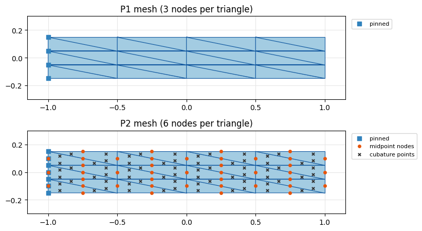
Both element sets live on the same coarse grid. linear_to_quadratic_elements keeps the P1 corners and appends one node per unique edge at its midpoint (\(T_2\) is \(t \times 6\)), and gauss_legendre_quadrature places symmetric cubature points (barycentric coordinates plus physical weights) inside every element. The figure shows the P1 mesh, and the P2 mesh with its midpoint nodes and cubature points; blue squares are the pinned left edge. The printout shows the cost: on the same 24 triangles P2 has 63 nodes (126 dofs) against P1’s 20 (40 dofs), with 3 cubature points per element.

V, T = igl.triangulated_grid(BEAM_NX, BEAM_NY)                       # unit square grid
X = (V - 0.5) * np.array([BEAM_WIDTH, BEAM_HEIGHT])                  # centred beam
V2, T2 = simkit.linear_to_quadratic_elements(X, T)                   # corners first, then edge midpoints
bary, w = simkit.gauss_legendre_quadrature(X, T, QUAD_ORDER)         # (t, n_quad, 3), (t, n_quad)
pin1 = np.where(X[:, 0] <= X[:, 0].min() + 1e-6)[0]
pin2 = np.where(V2[:, 0] <= V2[:, 0].min() + 1e-6)[0]
cub_rest = np.einsum("tqc,tcd->tqd", bary, X[T]).reshape(-1, 2)      # cubature points in the rest shape
n1, n2 = len(X), len(V2)
print(f"P1: {n1} nodes, {len(T)} elements, {2 * n1} dofs")
print(f"P2: {n2} nodes, {len(T2)} elements, {2 * n2} dofs, {bary.shape[1]} cubature points per element")

fig, axes = plt.subplots(2, 1, figsize=(9, 4.6))
lims = utils.auto_limits([X], pad=0.15)
utils.plot_mesh(axes[0], X, T, pins=pin1, lims=lims, title="P1 mesh (3 nodes per triangle)")
utils.plot_mesh(axes[1], V2, T2[:, :3], pins=pin2, lims=lims, title="P2 mesh (6 nodes per triangle)")
axes[1].scatter(V2[n1:, 0], V2[n1:, 1], s=16, color=utils.HANDLE_C, zorder=4, label="midpoint nodes")
axes[1].scatter(cub_rest[:, 0], cub_rest[:, 1], s=14, marker="x", color="0.2", zorder=4, label="cubature points")
for ax in axes:
    ax.legend(loc="upper left", bbox_to_anchor=(1.01, 1.0), fontsize=8)
fig.tight_layout()
simkit.filesystem.save_figure(fig, os.path.join(RESULTS_DIR, "beam_meshes.png"),
                              copy_to=os.path.join(MEDIA_DIR, "012_beam_meshes.png"))
plt.show()

P1: 20 nodes, 24 elements, 40 dofs
P2: 63 nodes, 24 elements, 126 dofs, 3 cubature points per element

Two operator sets, one energy

With P1 the energy is a one-point rule per element; with P2 it becomes a sum over cubature points,

\[E_{P1} = \sum_t \text{vol}_t\, \psi(F_t), \qquad E_{P2} = \sum_t \sum_q w_{tq}\, \psi(F_{tq}),\]

so no energy code changes: each cubature point is a pseudo-element whose weight w replaces vol. deformation_jacobian_p2 is still a constant sparse matrix, now mapping nodal positions to one \(F\) per cubature point (P2 shape-function gradients vary linearly inside the element), and P2 gets its own consistent mass matrix and gravity force; the printout checks the shapes, and that weights and masses integrate the beam’s area.

ops_p1 = dict(nodes=X, pins=pin1,
              J=simkit.deformation_jacobian(X, T),                                    # one F per element
              vol=simkit.volume(X, T),                                                # element areas
              M=sp.sparse.kron(simkit.massmatrix(X, T, rho=RHO), sp.sparse.eye(2)).tocsc(),
              f_g=simkit.gravity_force(X, T, a=GRAVITY, rho=RHO).reshape(-1, 1))
ops_p2 = dict(nodes=V2, pins=pin2,
              J=simkit.deformation_jacobian_p2(V2, T2, bary, w),                      # one F per cubature point
              vol=w.reshape(-1, 1),                                                   # cubature weights
              M=sp.sparse.kron(simkit.p2_massmatrix(V2, T2, bary, w, rho=RHO), sp.sparse.eye(2)).tocsc(),
              f_g=simkit.p2_gravity_force(V2, T2, bary, w, a=GRAVITY, rho=RHO).reshape(-1, 1))
for name, ops in (("P1", ops_p1), ("P2", ops_p2)):
    print(f"{name}: J {ops['J'].shape} -> {ops['J'].shape[0] // 4} F blocks, "
          f"sum of weights = {ops['vol'].sum():.4f} (area {BEAM_WIDTH * BEAM_HEIGHT:.4f}), "
          f"total mass = {ops['M'].sum() / 2:.4f}")

P1: J (96, 40) -> 24 F blocks, sum of weights = 0.6000 (area 0.6000), total mass = 0.6000
P2: J (288, 126) -> 72 F blocks, sum of weights = 0.6000 (area 0.6000), total mass = 0.6000

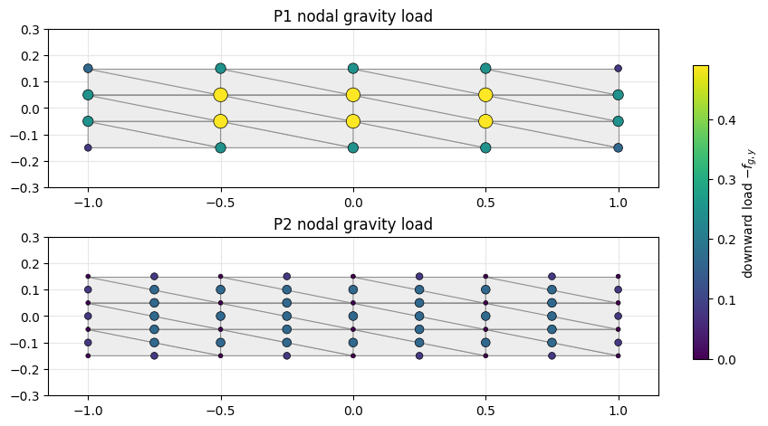
The consistent gravity load of every node, \(f_i = \int N_i\, \rho g \, dA\) (downward component, shown by colour and marker size on one scale for both). P1 spreads the beam’s weight over its corners in proportion to their adjacent area, but under uniform gravity the P2 corner nodes carry exactly zero load, because \(\int_t L_i(2L_i - 1)\, dA = 0\) on every triangle, and the edge midpoints carry all of it, as the printout confirms.

load = {name: -ops["f_g"].reshape(-1, 2)[:, 1] for name, ops in (("P1", ops_p1), ("P2", ops_p2))}  # downward load per node
print(f"P1: corner nodes carry {load['P1'].sum():.4f}   (beam weight {-RHO * GRAVITY * BEAM_WIDTH * BEAM_HEIGHT:.4f})")
print(f"P2: corner nodes carry {load['P2'][:n1].sum():.1e}, midpoint nodes carry {load['P2'][n1:].sum():.4f}")

fig, axes = plt.subplots(2, 1, figsize=(9, 4.6), layout="constrained")
lims = utils.auto_limits([X], pad=0.15)
vmax = max(load["P1"].max(), load["P2"].max())                       # shared colour scale
for ax, (name, nodes, tris) in zip(axes, (("P1", X, T), ("P2", V2, T2[:, :3]))):
    utils.plot_mesh(ax, nodes, tris, lims=lims, facecolor="0.93", edgecolor="0.55",
                    title=f"{name} nodal gravity load")
    m = ax.scatter(nodes[:, 0], nodes[:, 1], c=load[name], s=12 + 110 * load[name] / vmax, cmap="viridis",
                   vmin=0.0, vmax=vmax, edgecolors="k", linewidths=0.5, zorder=5)
fig.colorbar(m, ax=axes, shrink=0.8, label=r"downward load $-f_{g,y}$")
simkit.filesystem.save_figure(fig, os.path.join(RESULTS_DIR, "gravity_load.png"),
                              copy_to=os.path.join(MEDIA_DIR, "012_gravity_load.png"))
plt.show()

P1: corner nodes carry 5.8800   (beam weight 5.8800)
P2: corner nodes carry -3.3e-16, midpoint nodes carry 5.8800

The beam system

beam_system builds a hyperelastic (MATERIAL) beam from whichever operators it is handed; it cannot tell P1 from P2. Its terms are the elastic energy, the soft pin on the left edge, gravity, and, when the previous positions x_curr, x_prev are passed, the backward-Euler inertia term (one implicit step). Without them it is the static potential used for the equilibrium comparison later.

def beam_system(nodes, pins, J, vol, M, f_g, x_curr=None, x_prev=None):
    """Elastic + soft pin + gravity (+ backward-Euler inertia if x_curr, x_prev are given)."""
    n, dim = nodes.shape
    mu, lam = simkit.ympr_to_lame(YM, PR)
    mu = np.full((vol.shape[0], 1), mu)
    lam = np.full((vol.shape[0], 1), lam)
    Q_pin, b_pin = simkit.dirichlet_penalty(pins, nodes[pins], n, K_PIN)
    dynamic = x_curr is not None

    def energy_func(x):
        E_elastic = simkit.energies.elastic_energy_x(x.reshape(n, dim), J, mu, lam, vol, MATERIAL)
        E_pin = simkit.energies.quadratic_energy(x, Q_pin, b_pin)
        E_gravity = -(f_g.T @ x).item()
        E_inertia = simkit.energies.kinetic_energy_be(x, x_curr, x_prev, M, DT) if dynamic else 0.0
        E_total = E_elastic + E_pin + E_gravity + E_inertia
        return E_total

    def gradient_func(x):
        g_elastic = simkit.energies.elastic_gradient_x(x.reshape(n, dim), J, mu, lam, vol, MATERIAL)
        g_pin = simkit.energies.quadratic_gradient(x, Q_pin, b_pin)
        g_gravity = -f_g
        g_inertia = simkit.energies.kinetic_gradient_be(x, x_curr, x_prev, M, DT) if dynamic else 0.0
        g_total = g_elastic + g_pin + g_gravity + g_inertia
        return g_total

    def hessian_func(x):
        H_elastic = simkit.energies.elastic_hessian_x(x.reshape(n, dim), J, mu, lam, vol, MATERIAL, psd=True)
        H_pin = simkit.energies.quadratic_hessian(Q_pin)
        H_inertia = simkit.energies.kinetic_hessian_be(M, DT) if dynamic else 0.0
        H_total = H_elastic + H_pin + H_inertia
        return H_total

    return energy_func, gradient_func, hessian_func

Before simulating, we check gradient_func against a central-difference gradient of energy_func (simkit.gradient_cfd) at a randomly perturbed state, for both element sets with inertia switched on. Relative errors near \(10^{-8}\) or below mean the analytic gradient is right.

rng = np.random.default_rng(SEED)
for name, ops in (("P1", ops_p1), ("P2", ops_p2)):
    x_rest = ops["nodes"].reshape(-1, 1)
    energy_func, gradient_func, _ = beam_system(**ops, x_curr=x_rest, x_prev=x_rest)
    x_test = x_rest + FD_NOISE * rng.standard_normal(x_rest.shape)
    g_fd = simkit.gradient_cfd(lambda y: np.array(energy_func(y.reshape(-1, 1))), x_test.ravel(), FD_STEP)
    g = gradient_func(x_test).ravel()
    print(f"{name}: relative gradient error = {np.linalg.norm(g - g_fd) / np.linalg.norm(g):.2e}")

P1: relative gradient error = 8.25e-09
P2: relative gradient error = 1.66e-08

Curved (true-geometry) rendering of P2 elements

A P2 edge between corners \(a, b\) with midpoint node \(m\) is a parabola in the edge parameter \(t \in [0, 1]\):

\[x(t) = (1-t)(1-2t)\, U_a + t(2t-1)\, U_b + 4t(1-t)\, U_m .\]

This is just simkit.p2_shape_functions restricted to the edge, so we evaluate them at EDGE_SAMPLES barycentric points along each of the three edges. p2_curved_outline maps those samples through every element’s six nodes and returns the points plus one polygon per element, so the ordinary mesh drawing helpers can show the real curved boundary, which no straight-edged (P1) element can produce.

edge_t = np.linspace(0.0, 1.0, EDGE_SAMPLES)[:, None]
I3 = np.eye(3)
L_edges = np.vstack([(1 - edge_t) * I3[a] + edge_t * I3[b] for a, b in [(0, 1), (1, 2), (2, 0)]])  # barycentric samples on the 3 edges
N_edges = np.array([simkit.p2_shape_functions(Lk, 3)[0] for Lk in L_edges])                      # (3*S, 6) P2 basis on the edges

def p2_curved_outline(U2, T2):
    """Sample every P2 element's parabolic edges: points (t*3*S, 2) and polygons (t, 3*S)."""
    points = np.einsum("pi,tid->tpd", N_edges, U2[T2]).reshape(-1, 2)
    polygons = np.arange(len(points)).reshape(len(T2), -1)
    return points, polygons

Running both beams

Each beam takes T_TOTAL / DT backward-Euler steps: rebuild beam_system with the current and previous positions, then minimize it with Newton. We keep N_FRAMES evenly spaced frames and the height of the lowest point at every step. In the animation P1 is drawn with its straight triangles and P2 with its true curved edges: same mesh, material and timestep, yet only the P2 beam bends smoothly.

n_steps = int(round(T_TOTAL / DT))
frame_steps = set(np.round(np.linspace(0, n_steps, N_FRAMES)).astype(int))
frames, tip_y = {}, {}
for name, ops in (("P1", ops_p1), ("P2", ops_p2)):
    x_curr = ops["nodes"].reshape(-1, 1).copy()
    x_prev = x_curr.copy()                                            # starts at rest
    frames[name], tip_y[name] = [ops["nodes"].copy()], [ops["nodes"][:, 1].min()]
    for step in range(1, n_steps + 1):
        energy_func, gradient_func, hessian_func = beam_system(**ops, x_curr=x_curr, x_prev=x_prev)
        x_next = simkit.solvers.newton_solver(x_curr.copy(), energy_func, gradient_func, hessian_func,
                                              max_iter=STEP_ITERS, tolerance=STEP_TOL)
        x_prev, x_curr = x_curr, x_next
        tip_y[name].append(x_curr.reshape(-1, 2)[:, 1].min())
        if step in frame_steps:
            frames[name].append(x_curr.reshape(-1, 2).copy())

_, curved_polys = p2_curved_outline(V2, T2)
curved_p2 = [p2_curved_outline(U, T2)[0] for U in frames["P2"]]
fig, anim = utils.animate_meshes_grid(
    [{"states": frames["P1"], "T": T, "title": "Linear (P1) - straight edges"},
     {"states": curved_p2, "T": curved_polys, "title": "Quadratic (P2) - true curved edges"}],
    lims=utils.auto_limits(frames["P1"] + curved_p2, pad=0.15), fps=FPS, figsize=(9.4, 4.6),
    suptitle="Same mesh, same material, same dt: only P2's edges can curve")
fig.tight_layout()
video = simkit.filesystem.save_animation(anim, os.path.join(RESULTS_DIR, "p1_vs_p2_beam.mp4"), fps=FPS,
                                         copy_to=os.path.join(MEDIA_DIR, "012_p1_vs_p2_beam.mp4"))
plt.close(fig)
utils.embed_video(video)

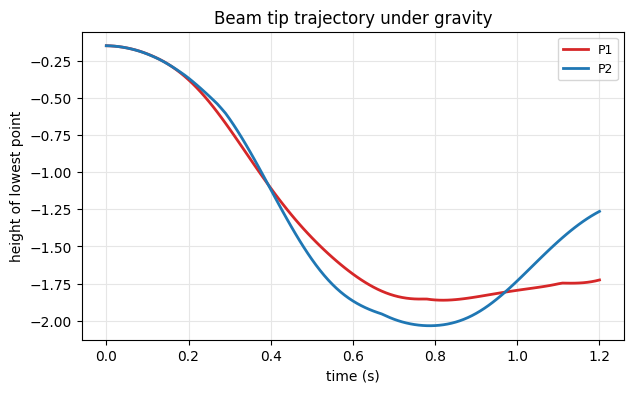
The height of the lowest point over time makes the comparison quantitative: the softer P2 beam falls further and then rebounds (at the end it whips back up, as in the last frames above), while the stiff P1 beam bottoms out higher and barely rebounds; the curves drift apart as the beams go out of phase.

times = DT * np.arange(n_steps + 1)
fig, ax = utils.line_plot(times, {"P1": tip_y["P1"], "P2": tip_y["P2"]}, colors=COLORS,
                          xlabel="time (s)", ylabel="height of lowest point",
                          title="Beam tip trajectory under gravity", figsize=(7, 4))
for name in tip_y:
    print(f"{name}: lowest point {min(tip_y[name]):.3f} at t = {DT * np.argmin(tip_y[name]):.2f} s")
simkit.filesystem.save_figure(fig, os.path.join(RESULTS_DIR, "tip_trajectory.png"),
                              copy_to=os.path.join(MEDIA_DIR, "012_tip_trajectory.png"))
plt.show()

P1: lowest point -1.862 at t = 0.82 s
P2: lowest point -2.034 at t = 0.79 s

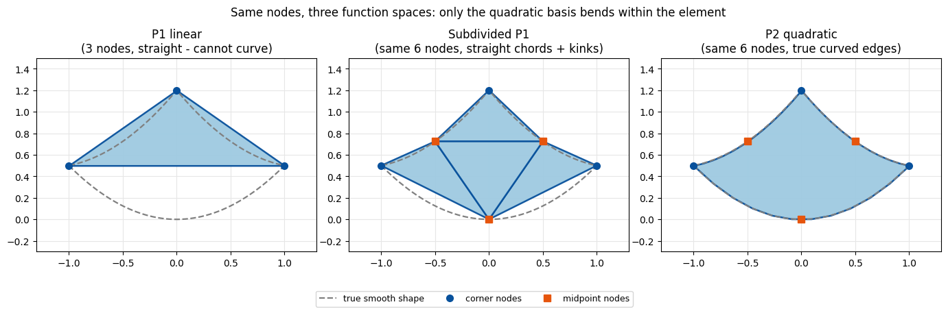
Wait — is this just a subdivided mesh?

A P2 element and a triangle subdivided into 4 linear sub-triangles use the same 6 nodes; the difference is the function space (table). Below, one triangle is deformed by the quadratic bending field \(\phi(x, y) = (x,\ y + \beta x^2)\), \(\beta =\) BEND, and drawn three ways: P1 stays flat, subdivision is a kinked chord, and only the quadratic basis matches the true shape (dashed grey), which is why P2 reproduces quadratic fields exactly while no linear scheme on these nodes can.

scheme	nodes	within an element	edges
P1 linear	3 corners	constant \(F\)	straight
Subdivided P1	same 6	piecewise-constant \(F\), kinks at midpoints	straight chords
P2 quadratic	same 6	\(F\) varies linearly and smoothly	curved (parabolic)

def phi(P):
    """Quadratic bending field phi(x, y) = (x, y + BEND x^2)."""
    P = np.atleast_2d(P)
    return np.column_stack([P[:, 0], P[:, 1] + BEND * P[:, 0] ** 2])

corners = DEMO_CORNERS
node6 = np.vstack([corners, 0.5 * (corners + np.roll(corners, -1, axis=0))])   # [c0, c1, c2, m01, m12, m20]
U6 = phi(node6)
s = np.linspace(0, 1, TRUTH_SAMPLES)[:, None]
truth = phi(np.vstack([(1 - s) * corners[i] + s * corners[(i + 1) % 3] for i in range(3)]))  # true outline
T_sub = np.array([[0, 3, 5], [3, 1, 4], [5, 4, 2], [3, 4, 5]])                 # 4-way subdivision
P_curved, poly_curved = p2_curved_outline(U6, np.array([[0, 1, 2, 3, 4, 5]]))
panels = [("P1 linear\n(3 nodes, straight - cannot curve)", U6[:3], np.array([[0, 1, 2]])),
          ("Subdivided P1\n(same 6 nodes, straight chords + kinks)", U6, T_sub),
          ("P2 quadratic\n(same 6 nodes, true curved edges)", P_curved, poly_curved)]

lims = utils.auto_limits([truth, U6], pad=0.3)
fig, axes = plt.subplots(1, 3, figsize=(13.8, 4.5))
for ax, (title, P, F) in zip(axes, panels):
    utils.plot_mesh(ax, P, F, lims=lims, title=title, lw=1.8)
    ax.plot(np.r_[truth[:, 0], truth[0, 0]], np.r_[truth[:, 1], truth[0, 1]],
            color="0.5", lw=1.6, ls="--", zorder=4, label="true smooth shape")
    ax.plot(U6[:3, 0], U6[:3, 1], "o", color=utils.MESH_EDGE, ms=7, zorder=5, label="corner nodes")
    if ax is not axes[0]:
        ax.plot(U6[3:, 0], U6[3:, 1], "s", color=utils.HANDLE_C, ms=7, zorder=5, label="midpoint nodes")
fig.legend(*axes[1].get_legend_handles_labels(), loc="lower center", ncol=3, fontsize=9)
fig.suptitle("Same nodes, three function spaces: only the quadratic basis bends within the element", fontsize=12)
fig.tight_layout(rect=(0, 0.07, 1, 1))
simkit.filesystem.save_figure(fig, os.path.join(RESULTS_DIR, "p1_vs_subdivided_vs_p2.png"),
                              copy_to=os.path.join(MEDIA_DIR, "012_p1_vs_subdivided_vs_p2.png"))
plt.show()

Static equilibrium: the unambiguous stiffness comparison

The animation includes inertia, so at any instant both beams are still swinging (slightly out of phase, since their mass distributions differ). To compare stiffness cleanly we build beam_system without the inertia term and solve for the gravity equilibrium each beam eventually settles into. The clip alternates between rest and equilibrium; linear triangles cannot bend within an element, so P1 is artificially stiff and deflects less.

eq, newton_grad = {}, {}
for name, ops in (("P1", ops_p1), ("P2", ops_p2)):
    energy_func, gradient_func, hessian_func = beam_system(**ops)                # static: no inertia
    x_eq, info = simkit.solvers.newton_solver(ops["nodes"].reshape(-1, 1).copy(), energy_func, gradient_func,
                                              hessian_func, max_iter=STATIC_ITERS, tolerance=STATIC_TOL,
                                              return_info=True)
    eq[name] = x_eq.reshape(-1, 2)
    newton_grad[name] = [np.linalg.norm(g) for g in info["g"]] + [np.linalg.norm(gradient_func(x_eq))]
y_rest = X[:, 1].min()                                                          # lowest point at rest
tip = {name: y_rest - eq[name][:, 1].min() for name in eq}                      # downward tip deflection
print(f"P1 tip deflection: {tip['P1']:.4f}")
print(f"P2 tip deflection: {tip['P2']:.4f}   (P2 is {100 * (tip['P2'] - tip['P1']) / tip['P1']:.1f}% more compliant)")

curved_static = [p2_curved_outline(U, T2)[0] for U in (V2, eq["P2"])]
fig, anim = utils.animate_meshes_grid(
    [{"states": [X, eq["P1"]], "T": T, "title": f"P1 equilibrium (tip deflection {tip['P1']:.3f})"},
     {"states": curved_static, "T": curved_polys, "title": f"P2 equilibrium (tip deflection {tip['P2']:.3f}, curved)"}],
    lims=utils.auto_limits([X, eq["P1"]] + curved_static, pad=0.15), fps=STATIC_FPS, figsize=(9.4, 4.6),
    suptitle="Static gravity equilibrium: linear elements are stiffer (deflect less)")
fig.tight_layout()
video = simkit.filesystem.save_animation(anim, os.path.join(RESULTS_DIR, "p1_vs_p2_static.mp4"), fps=STATIC_FPS,
                                         copy_to=os.path.join(MEDIA_DIR, "012_p1_vs_p2_static.mp4"))
plt.close(fig)
utils.embed_video(video)

P1 tip deflection: 1.2620
P2 tip deflection: 1.7120   (P2 is 35.7% more compliant)

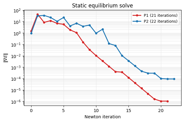
As a solver check, the gradient norm per Newton iteration of both static solves. After the line-searched large-deformation phase it falls by roughly 5 (P2) to 7 (P1) orders of magnitude from its peak, until the Newton step is below STATIC_TOL. The tail is linear rather than quadratic because psd=True projects each element Hessian to be positive semi-definite, which only approximates the true Hessian where elements are compressed.

labels = {name: f"{name} ({len(g) - 1} iterations)" for name, g in newton_grad.items()}
fig, ax = utils.residual_plot({labels[name]: g for name, g in newton_grad.items()},
                              colors={labels[name]: COLORS[name] for name in labels}, markers=True, stagger=False,
                              xlabel="Newton iteration", ylabel=r"$\|\nabla E\|$",
                              title="Static equilibrium solve", figsize=(6.5, 4))
simkit.filesystem.save_figure(fig, os.path.join(RESULTS_DIR, "static_newton.png"),
                              copy_to=os.path.join(MEDIA_DIR, "012_static_newton.png"))
plt.show()

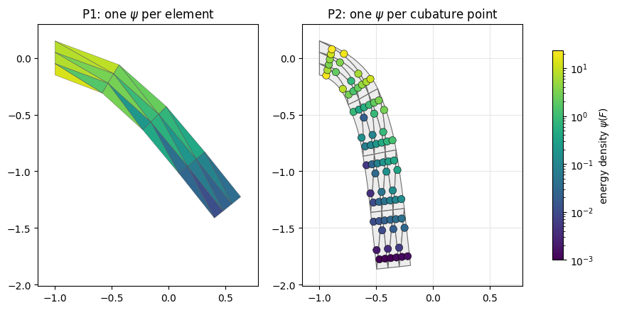
The elastic energy density \(\psi(F)\) at equilibrium shows why P1 is stiff. P1 has one \(F\), hence one \(\psi\), per triangle (flat colours); P2 has one per cubature point (dots at their deformed positions), so the strain varies inside each element and the curvature is carried smoothly instead of being forced into piecewise-constant pieces. Both panels share one logarithmic colour scale.

mu, lam = simkit.ympr_to_lame(YM, PR)
psi = {}
for name, ops in (("P1", ops_p1), ("P2", ops_p2)):
    F = (ops["J"] @ eq[name].reshape(-1, 1)).reshape(-1, 2, 2)                     # one F per block
    n_blocks = len(F)
    psi[name] = simkit.energies.elastic_energy_element_F(F, np.full((n_blocks, 1), mu),
                                                         np.full((n_blocks, 1), lam), MATERIAL).ravel()
N_quad = np.array([simkit.p2_shape_functions(Lq, 3)[0] for Lq in bary[0]])          # (n_quad, 6), same rule per element
cub_eq = np.einsum("qi,tid->tqd", N_quad, eq["P2"][T2]).reshape(-1, 2)              # deformed cubature points
norm = LogNorm(vmin=1e-3, vmax=max(psi["P1"].max(), psi["P2"].max()))

fig, axes = plt.subplots(1, 2, figsize=(11, 4.8))
lims = utils.auto_limits([eq["P1"], eq["P2"]], pad=0.15)
utils.plot_scalar_field(axes[0], eq["P1"], T, np.maximum(psi["P1"], norm.vmin), lims=lims, norm=norm,
                        title="P1: one $\\psi$ per element", colorbar=False)
utils.plot_mesh(axes[1], p2_curved_outline(eq["P2"], T2)[0], curved_polys, lims=lims,
                facecolor="0.93", edgecolor="0.4", title="P2: one $\\psi$ per cubature point")
m = axes[1].scatter(cub_eq[:, 0], cub_eq[:, 1], c=np.maximum(psi["P2"], norm.vmin), s=55, norm=norm,
                    edgecolors="k", linewidths=0.4, zorder=6)
fig.colorbar(m, ax=axes, shrink=0.8, label=r"energy density $\psi(F)$")
simkit.filesystem.save_figure(fig, os.path.join(RESULTS_DIR, "energy_density.png"),
                              copy_to=os.path.join(MEDIA_DIR, "012_energy_density.png"))
plt.show()

Part C — Convergence: P1 is first order, P2 is second order

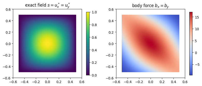
The real payoff of quadratic elements is accuracy per refinement. With the method of manufactured solutions we pick the exact displacement \(u^*(x,y) = (s, s)\), \(s = \sin(\pi a)\sin(\pi b)\), \(a = x + \tfrac12\), \(b = y + \tfrac12\) on the unit square (zero on the boundary), and derive the body force \(b = -\operatorname{div}\sigma(u^*) = -\mu\Delta u^* - (\mu + \lambda)\nabla(\nabla\cdot u^*)\) that makes it the solution of linear elasticity (a linear PDE, so the rates are textbook-clean). Below: the exact field \(s\) and the body force component \(b_x\) on the finest mesh.

mms_mu, mms_lam = simkit.ympr_to_lame(MMS_YM, MMS_PR)

def u_star(P):
    """Exact displacement (s, s); zero on the boundary."""
    a, b = P[..., 0] + 0.5, P[..., 1] + 0.5
    s = np.sin(np.pi * a) * np.sin(np.pi * b)
    return np.stack([s, s], axis=-1)

def grad_u_star(P):
    """Exact displacement gradient at one point: rows = component i, cols = d/dX_j."""
    a, b = P[0] + 0.5, P[1] + 0.5
    sx = np.pi * np.cos(np.pi * a) * np.sin(np.pi * b)
    sy = np.pi * np.sin(np.pi * a) * np.cos(np.pi * b)
    return np.array([[sx, sy], [sx, sy]])

def body_force(P):
    """b = -mu Lap(u*) - (mu + lam) grad(div u*), at one point."""
    a, b = P[0] + 0.5, P[1] + 0.5
    s = np.sin(np.pi * a) * np.sin(np.pi * b)
    c = np.cos(np.pi * a) * np.cos(np.pi * b)
    b_shear = 2 * mms_mu * np.pi ** 2 * s                                # -mu Lap(u*)
    b_volumetric = -(mms_mu + mms_lam) * np.pi ** 2 * (c - s)            # -(mu + lam) grad(div u*)
    b_total = b_shear + b_volumetric
    return np.array([b_total, b_total])

mms_meshes = {}
for nn in MMS_RESOLUTIONS:
    V_unit, T_mms = igl.triangulated_grid(nn + 1, nn + 1)
    mms_meshes[nn] = (V_unit - 0.5, T_mms)                                   # unit square [-1/2, 1/2]^2
X_fine, T_fine = mms_meshes[MMS_RESOLUTIONS[-1]]
fig, axes = plt.subplots(1, 2, figsize=(10, 4.2))
utils.plot_scalar_field(axes[0], X_fine, T_fine, u_star(X_fine)[:, 0], edges=False, title="exact field $s = u^*_x = u^*_y$")
utils.plot_scalar_field(axes[1], X_fine, T_fine, [body_force(p)[0] for p in X_fine], edges=False,
                        cmap="coolwarm", title="body force $b_x = b_y$")
simkit.filesystem.save_figure(fig, os.path.join(RESULTS_DIR, "mms_solution.png"),
                              copy_to=os.path.join(MEDIA_DIR, "012_mms_solution.png"))
plt.show()

The finite-element pieces, identical for P1 and P2 apart from the shape functions:

• assemble_load: the consistent load \(f_i = \int N_i\, b \, dV\) by quadrature.

• mms_system: linear elasticity + a stiff \(u = 0\) boundary pin + the load potential \(-f^\top x\). It is quadratic, so a single undamped Newton step from rest is the exact solve.

• error_norms: the L2 displacement error \(\lVert u_h - u^*\rVert\) and the H1 (strain) seminorm error \(\lVert \nabla u_h - \nabla u^*\rVert\), integrated by quadrature (with \(\nabla u_h = F - I\)).

def assemble_load(nodes, T_el, bary, weights, shape_at):
    """Consistent load vector f_i = integral N_i b dV, by quadrature."""
    f = np.zeros(nodes.shape)
    for e in range(len(T_el)):
        X_corners = nodes[T_el[e, :3]]                                   # corners -> affine rest map
        for q in range(bary.shape[1]):
            L_q = bary[e, q]
            N = shape_at(L_q)
            b_q = body_force(L_q @ X_corners)
            for i, node in enumerate(T_el[e]):
                f[node] += weights[e, q] * N[i] * b_q
    return f

def mms_system(nodes, J, vol, f_load, bnd):
    """Linear elasticity + stiff boundary pin (u = 0) + body-force load, in stacked positions x."""
    n, dim = nodes.shape
    mu = np.full((vol.shape[0], 1), mms_mu)
    lam = np.full((vol.shape[0], 1), mms_lam)
    Q_pin, b_pin = simkit.dirichlet_penalty(bnd, nodes[bnd], n, MMS_K_PIN)
    f = f_load.reshape(-1, 1)

    def energy_func(x):
        E_elastic = simkit.energies.elastic_energy_x(x.reshape(n, dim), J, mu, lam, vol, "linear-elasticity")
        E_pin = simkit.energies.quadratic_energy(x, Q_pin, b_pin)
        E_load = -(f.T @ x).item()
        E_total = E_elastic + E_pin + E_load
        return E_total

    def gradient_func(x):
        g_elastic = simkit.energies.elastic_gradient_x(x.reshape(n, dim), J, mu, lam, vol, "linear-elasticity")
        g_pin = simkit.energies.quadratic_gradient(x, Q_pin, b_pin)
        g_load = -f
        g_total = g_elastic + g_pin + g_load
        return g_total

    def hessian_func(x):
        H_elastic = simkit.energies.elastic_hessian_x(x.reshape(n, dim), J, mu, lam, vol, "linear-elasticity")
        H_pin = simkit.energies.quadratic_hessian(Q_pin)
        H_total = H_elastic + H_pin
        return H_total

    return energy_func, gradient_func, hessian_func

def error_norms(nodes, T_el, x, bary, weights, F, shape_at):
    """L2 displacement error and H1 (strain) seminorm error against the exact field."""
    l2_sq, h1_sq = 0.0, 0.0
    for e in range(len(T_el)):
        X_corners = nodes[T_el[e, :3]]
        u_el = x[T_el[e]] - nodes[T_el[e]]                               # nodal displacements
        for q in range(bary.shape[1]):
            x_q = bary[e, q] @ X_corners
            u_h = shape_at(bary[e, q]) @ u_el                            # interpolated FE displacement
            l2_sq += weights[e, q] * np.sum((u_h - u_star(x_q)) ** 2)
            h1_sq += weights[e, q] * np.sum((F[e, q] - np.eye(2) - grad_u_star(x_q)) ** 2)
    return np.sqrt(l2_sq), np.sqrt(h1_sq)

P1_SHAPE = lambda L: L                                                   # linear hats = barycentric coordinates
P2_SHAPE = lambda L: simkit.p2_shape_functions(L, 3)[0]                  # quadratic shape functions

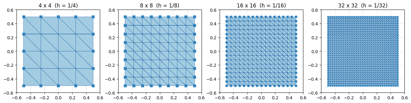
The refinement sequence. Every boundary node (blue) is pinned to \(u = 0\); P2 uses the same meshes plus their edge midpoints.

fig, axes = plt.subplots(1, len(MMS_RESOLUTIONS), figsize=(3.3 * len(MMS_RESOLUTIONS), 3.4))
for ax, (nn, (Xm, Tm)) in zip(axes, mms_meshes.items()):
    bnd = np.where(np.abs(Xm).max(axis=1) > 0.5 - 1e-9)[0]
    utils.plot_mesh(ax, Xm, Tm, lw=0.5, title=f"{nn} x {nn}  (h = 1/{nn})")
    ax.scatter(Xm[bnd, 0], Xm[bnd, 1], s=min(28, 240 / nn), marker="s", color=utils.PIN_C, zorder=4)
fig.tight_layout()
simkit.filesystem.save_figure(fig, os.path.join(RESULTS_DIR, "mms_meshes.png"),
                              copy_to=os.path.join(MEDIA_DIR, "012_mms_meshes.png"))
plt.show()

Refinement sweep

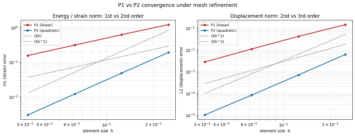
On each mesh we solve the manufactured problem with P1 and with P2 (order MMS_STIFF_QUAD_ORDER cubature for the stiffness, exact here because P2 strains are linear; order MMS_QUAD_ORDER for load and errors) and record both error norms. The printed orders are the slopes of \(\log(\text{error})\) against \(\log h\).

hs = np.array([1.0 / nn for nn in MMS_RESOLUTIONS])
err = {"P1 L2": [], "P1 H1": [], "P2 L2": [], "P2 H1": []}
solutions = {}
for nn in MMS_RESOLUTIONS:
    Xm, Tm = mms_meshes[nn]
    bq, wq = simkit.gauss_legendre_quadrature(Xm, Tm, MMS_QUAD_ORDER)   # accurate load + error quadrature

    # --- P1 ---
    J1, vol1 = simkit.deformation_jacobian(Xm, Tm), simkit.volume(Xm, Tm)
    f1 = assemble_load(Xm, Tm, bq, wq, P1_SHAPE)
    bnd1 = np.where(np.abs(Xm).max(axis=1) > 0.5 - 1e-9)[0]
    energy_func, gradient_func, hessian_func = mms_system(Xm, J1, vol1, f1, bnd1)
    x1 = simkit.solvers.newton_solver(Xm.reshape(-1, 1).copy(), energy_func, gradient_func, hessian_func,
                                      max_iter=1, do_line_search=False).reshape(-1, 2)
    F1 = np.repeat(simkit.deformation_gradient(Xm, Tm, x1)[:, None], bq.shape[1], axis=1)
    l2, h1 = error_norms(Xm, Tm, x1, bq, wq, F1, P1_SHAPE)
    err["P1 L2"].append(l2)
    err["P1 H1"].append(h1)

    # --- P2 ---
    Vm2, Tm2 = simkit.linear_to_quadratic_elements(Xm, Tm)
    b2, w2 = simkit.gauss_legendre_quadrature(Xm, Tm, MMS_STIFF_QUAD_ORDER)   # stiffness cubature
    J2, vol2 = simkit.deformation_jacobian_p2(Vm2, Tm2, b2, w2), w2.reshape(-1, 1)
    f2 = assemble_load(Vm2, Tm2, bq, wq, P2_SHAPE)
    bnd2 = np.where(np.abs(Vm2).max(axis=1) > 0.5 - 1e-9)[0]
    energy_func, gradient_func, hessian_func = mms_system(Vm2, J2, vol2, f2, bnd2)
    x2 = simkit.solvers.newton_solver(Vm2.reshape(-1, 1).copy(), energy_func, gradient_func, hessian_func,
                                      max_iter=1, do_line_search=False).reshape(-1, 2)
    F2 = simkit.deformation_gradient_p2(Vm2, Tm2, bq, x2)
    l2, h1 = error_norms(Vm2, Tm2, x2, bq, wq, F2, P2_SHAPE)
    err["P2 L2"].append(l2)
    err["P2 H1"].append(h1)
    solutions[nn] = (x1, x2)

slope = lambda e: np.polyfit(np.log(hs), np.log(e), 1)[0]
print(f"P1  H1 (strain) order = {slope(err['P1 H1']):.2f}   (theory 1)")
print(f"P2  H1 (strain) order = {slope(err['P2 H1']):.2f}   (theory 2)")
print(f"P1  L2 (displ.) order = {slope(err['P1 L2']):.2f}   (theory 2)")
print(f"P2  L2 (displ.) order = {slope(err['P2 L2']):.2f}   (theory 3)")

P1  H1 (strain) order = 0.99   (theory 1)
P2  H1 (strain) order = 1.99   (theory 2)
P1  L2 (displ.) order = 1.90   (theory 2)
P2  L2 (displ.) order = 3.07   (theory 3)

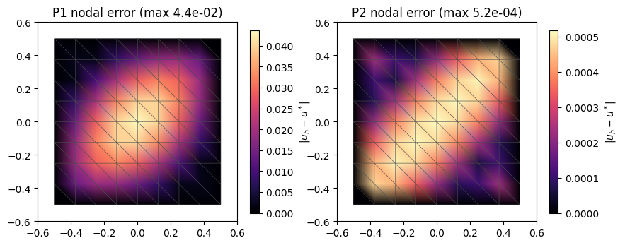
The pointwise displacement error \(|u_h - u^*|\) at the corner nodes of the MMS_SHOW_RES mesh (note the separate colour scales): on the same mesh P2 is roughly two orders of magnitude more accurate.

Xm, Tm = mms_meshes[MMS_SHOW_RES]
x1, x2 = solutions[MMS_SHOW_RES]
fig, axes = plt.subplots(1, 2, figsize=(10, 4.2))
for ax, (name, x) in zip(axes, (("P1", x1), ("P2", x2[:len(Xm)]))):
    node_err = np.linalg.norm(x - Xm - u_star(Xm), axis=1)
    utils.plot_scalar_field(ax, Xm, Tm, node_err, cmap="magma",
                            title=f"{name} nodal error (max {node_err.max():.1e})", label="$|u_h - u^*|$")
simkit.filesystem.save_figure(fig, os.path.join(RESULTS_DIR, "mms_error_fields.png"),
                              copy_to=os.path.join(MEDIA_DIR, "012_mms_error_fields.png"))
plt.show()

For a smooth solution and degree-\(p\) elements, theory predicts these rates, and the log-log plot confirms them (dashed guides). Halving \(h\) cuts P1’s strain error by ~2 but P2’s by ~4, so P2 reaches a target accuracy on a far coarser mesh.

norm	rate	P1 (\(p=1\))	P2 (\(p=2\))
H1 / strain	\(O(h^p)\)	\(O(h)\)	\(O(h^2)\)
L2 / displacement	\(O(h^{p+1})\)	\(O(h^2)\)	\(O(h^3)\)

colors = {"P1 (linear)": COLORS["P1"], "P2 (quadratic)": COLORS["P2"]}
fig, axes = plt.subplots(1, 2, figsize=(12.5, 4.8))
utils.loglog_plot(hs, {"P1 (linear)": err["P1 H1"], "P2 (quadratic)": err["P2 H1"]},
                  xlabel="element size  h", ylabel="H1 (strain) error", colors=colors,
                  ref_slopes={"O(h)": 1, "O(h^2)": 2},
                  title="Energy / strain norm: 1st vs 2nd order", ax=axes[0])
utils.loglog_plot(hs, {"P1 (linear)": err["P1 L2"], "P2 (quadratic)": err["P2 L2"]},
                  xlabel="element size  h", ylabel="L2 (displacement) error", colors=colors,
                  ref_slopes={"O(h^2)": 2, "O(h^3)": 3},
                  title="Displacement norm: 2nd vs 3rd order", ax=axes[1])
fig.suptitle("P1 vs P2 convergence under mesh refinement", fontsize=13)
fig.tight_layout()
simkit.filesystem.save_figure(fig, os.path.join(RESULTS_DIR, "convergence.png"),
                              copy_to=os.path.join(MEDIA_DIR, "012_convergence.png"))
plt.show()

Takeaways

• At static equilibrium the P1 beam is artificially stiff (it cannot bend within an element) and deflects less; P2 sags further and more smoothly, with strain varying inside each element.

• It is not a subdivided mesh: both use the same 6 nodes, but only the quadratic basis has genuinely curved (parabolic) edges and reproduces quadratic fields exactly.

• Convergence: P1 is first order and P2 second order in the strain (H1) norm, one order higher each in L2, so P2 reaches a target accuracy on a much coarser mesh.

• The elastic energy, gradient and Hessian code is unchanged: P2 only swaps \(J\) (one \(F\) per cubature point), the integration weights, and the mass/gravity assembly.