19 · Compressed Vibration Modes: trading global modes for local ones#
Linear modal analysis (LMA) solves \(H u = \omega^2 M u\) (stiffness \(H\), mass \(M\)) for the shapes an elastic body likes to vibrate in, but its low modes are global: on a beam they are standing waves over the whole length, a poor basis for editing, actuating or simulating a body part by part. Compressed modes (Brandt & Hildebrandt, 2017) add a mass-weighted \(L_1\) penalty that rewards shapes that are exactly zero almost everywhere. Each mode solves the problem below; \(\lambda = 0\) gives back LMA, and a larger \(\lambda\) gives a smaller support.
Imports, and every tunable parameter of this notebook.
%matplotlib inline
import os
import numpy as np
import scipy as sp
import matplotlib.pyplot as plt
import igl
import simkit
import utils

NOTEBOOK = "019_compressed_modes"                                  # this file's name
RESULTS_DIR = utils.notebook_results_path(NOTEBOOK)               # results/019_compressed_modes/
MEDIA_DIR = "media"                                                # tracked copies for the website
# mesh and material
NX, NY = 40, 6                   # grid resolution (vertices)
WIDTH, HEIGHT = 6.0, 0.9         # beam size
MU, LAM = 1.0, 1.0               # unit Lame parameters: only the mode *shapes* matter
RHO = 1.0                        # density of the lumped mass matrix
MATERIAL = "linear-elasticity"   # small-strain elasticity, so the stiffness H is constant
# modes
N_RIGID = 3                      # rigid-body modes of a free 2D body (2 translations + 1 rotation)
N_MODES = 5                      # deformation / compressed modes per basis
LAMBDAS = [0.5, 2.0, 8.0]        # L1 sparsity weights of the compressed-mode sweep
ICCM_ITERS = 25                  # max convex-QP iterations per compressed mode
ICCM_TOL = 1e-6                  # stop a mode when its objective decrement falls below this
SEED = 0                         # seed of each compressed mode's random start and of the checks
ACTIVE_THRESH = 0.05             # a vertex is "active" in a mode if it moves > 5% of the mode's peak
# checks
FD_STEP = 1e-6                   # central-difference step of the gradient checks
FD_NOISE = 0.05                  # size of the random displacement the checks run at
# animation
N_FRAMES = 36                    # frames per sine period
SCREEN_AMP = 0.32                # largest on-screen vertex displacement of every mode
FPS = 18                         # video frame rate
A free-standing beam#
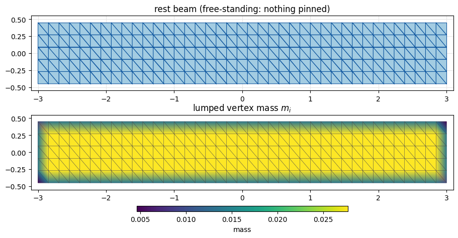
We mesh a long thin rectangle with igl.triangulated_grid and pin nothing, so the beam floats in space.
simkit.massmatrix lumps each triangle’s mass equally onto its corners (bottom panel): boundary vertices
carry less mass, corners the least. Expanded to one copy per \(x\)/\(y\) DOF, it is the mass \(M\) of both mode
problems, and its diagonal \(m_i\) also weights the \(L_1\) penalty. The printed total mass equals
WIDTH * HEIGHT * RHO = 5.4, so the lumping conserves mass.
V, T = igl.triangulated_grid(NX, NY)                         # unit square, NX x NY vertices
X = (V - 0.5) * np.array([WIDTH, HEIGHT])                    # centered WIDTH x HEIGHT rectangle
n, dim = X.shape
x_rest = X.reshape(-1, 1)                                    # stacked rest positions

M_vertex = simkit.massmatrix(X, T, rho=RHO)                  # lumped, diagonal (n, n)
M = sp.sparse.kron(M_vertex, sp.sparse.eye(dim)).tocsc()     # one copy per DOF, (n*dim, n*dim)
print(f"beam: {n} vertices, {len(T)} triangles, {n * dim} DOFs, total mass {M_vertex.sum():.2f}")

fig, axes = plt.subplots(2, 1, figsize=(9, 4.6), layout="constrained")
utils.plot_mesh(axes[0], X, T, title="rest beam (free-standing: nothing pinned)")
field = utils.plot_scalar_field(axes[1], X, T, M_vertex.diagonal(), title="lumped vertex mass $m_i$",
                                colorbar=False)
fig.colorbar(field, ax=axes[1], orientation="horizontal", shrink=0.5, aspect=40, label="mass")
simkit.filesystem.save_figure(fig, os.path.join(RESULTS_DIR, "beam.png"),
                              copy_to=os.path.join(MEDIA_DIR, "019_beam.png"))
plt.show()
beam: 240 vertices, 390 triangles, 480 DOFs, total mass 5.40
The elastic system#
free_beam_system is the beam’s mechanical system, built from simkit: small-strain elasticity evaluated on
\(F = Jx\) and weighted by triangle area. With nothing pinned it is the only term. Linear elasticity is
quadratic in \(x\), so its Hessian at rest is the stiffness \(H\) of both mode problems. It is already
positive semi-definite, so we take it exactly (psd=False).
def free_beam_system(X, T, material):
    """Elastic energy of an unpinned body, in stacked vertex positions x."""
    n, dim = X.shape
    J = simkit.deformation_jacobian(X, T)
    vol = simkit.volume(X, T)
    mu = np.full((len(T), 1), MU)
    lam = np.full((len(T), 1), LAM)

    def energy_func(x):
        E_elastic = simkit.energies.elastic_energy_x(x.reshape(n, dim), J, mu, lam, vol, material)
        E_total = E_elastic
        return E_total

    def gradient_func(x):
        g_elastic = simkit.energies.elastic_gradient_x(x.reshape(n, dim), J, mu, lam, vol, material)
        g_total = g_elastic
        return g_total

    def hessian_func(x):
        H_elastic = simkit.energies.elastic_hessian_x(x.reshape(n, dim), J, mu, lam, vol, material, psd=False)
        H_total = H_elastic
        return H_total

    return energy_func, gradient_func, hessian_func

beam_energy, beam_gradient, beam_hessian = free_beam_system(X, T, MATERIAL)
H = beam_hessian(x_rest).tocsc()                             # constant stiffness, (n*dim, n*dim)
The compressed-mode objective#
compressed_mode_system is the objective of one compressed mode in its displacement \(u\): the elastic term
\(\tfrac12 u^\top H u\) plus the sparsity term \(\lambda\, m^\top |u|\), with \(m\) the lumped mass of every DOF.
Away from \(u_i = 0\) the sparsity gradient is \(\lambda\, m \odot \operatorname{sign}(u)\) and its Hessian
vanishes. The kink at zero is what makes exact zeros optimal, and why Newton is the wrong tool:
simkit.eigs_iccm instead splits \(u = u_+ - u_-\) with \(u_\pm \ge 0\), which makes the \(L_1\) term linear, and
solves a convex QP per iteration. We use these closures to check and score its modes.
def compressed_mode_system(H, M, l):
    """Compressed-mode objective 0.5 u^T H u + l m^T |u| in a modal displacement u."""
    m = np.asarray(M.sum(axis=1)).reshape(-1, 1)             # lumped mass of every DOF
    b0 = np.zeros((H.shape[0], 1))                           # the elastic term has no linear part

    def energy_func(u):
        E_elastic = simkit.energies.quadratic_energy(u, H, b0)
        E_sparse = l * (m.T @ np.abs(u)).item()
        E_total = E_elastic + E_sparse
        return E_total

    def gradient_func(u):
        g_elastic = simkit.energies.quadratic_gradient(u, H, b0)
        g_sparse = l * m * np.sign(u)                        # a subgradient wherever some u_i = 0
        g_total = g_elastic + g_sparse
        return g_total

    def hessian_func(u):
        H_elastic = simkit.energies.quadratic_hessian(H)
        H_sparse = sp.sparse.csc_matrix(H.shape)             # |u| is piecewise linear: no curvature
        H_total = H_elastic + H_sparse
        return H_total

    return energy_func, gradient_func, hessian_func
Check both systems#
At a random displacement \(d\) (all entries nonzero, so \(|u|\) is differentiable there), central finite
differences (simkit.gradient_cfd) of each energy should match its gradient, and the beam energy should
equal \(\tfrac12 d^\top H d\), confirming that \(H\) captures the whole elastic energy.
rng = np.random.default_rng(SEED)
d = FD_NOISE * rng.standard_normal((n * dim, 1))             # random displacement
mode_energy, mode_gradient, mode_hessian = compressed_mode_system(H, M, LAMBDAS[-1])
checks = {"free_beam_system": (beam_energy, beam_gradient, x_rest + d),
          "compressed_mode_system": (mode_energy, mode_gradient, d)}
for name, (energy_func, gradient_func, y) in checks.items():
    g = gradient_func(y)
    g_fd = simkit.gradient_cfd(lambda z: np.array(energy_func(z.reshape(-1, 1))), y.ravel(), FD_STEP)
    rel_err = np.linalg.norm(g_fd.reshape(-1, 1) - g) / np.linalg.norm(g)
    print(f"{name:23s} |g_fd - g| / |g| = {rel_err:.1e}")
print(f"E(x_rest + d) = {beam_energy(x_rest + d):.12f}")
print(f"0.5 d^T H d   = {0.5 * (d.T @ (H @ d)).item():.12f}")
free_beam_system        |g_fd - g| / |g| = 5.3e-10
compressed_mode_system  |g_fd - g| / |g| = 5.1e-10
E(x_rest + d) = 4.159243608927
0.5 d^T H d   = 4.159243608927
Linear modal analysis: global modes#
simkit.eigs solves \(Hu = \omega^2 Mu\) for the lowest eigenpairs (what simkit.linear_modal_analysis does
for a unit material). The first three eigenvalues are \(\approx 0\): the rigid translations and rotation in the
null space of \(H\). We drop them and keep the next five, the deformation modes. active_fraction
measures locality: the share of (vertex, mode) pairs that move more than 5% of their mode’s peak. For LMA
it is 1: every mode moves every vertex.
def mode_magnitude(B):
    """Per-vertex displacement magnitude of every mode (column) of B, shape (n, k)."""
    return np.linalg.norm(B.reshape(n, dim, -1), axis=1)

def active_fraction(B):
    """Share of (vertex, mode) pairs that move more than ACTIVE_THRESH of their mode's peak."""
    mag = mode_magnitude(B)
    return (mag > ACTIVE_THRESH * mag.max(axis=0)).mean()

omega2, B_all = simkit.eigs(H, k=N_RIGID + N_MODES, M=M)
print("eigenvalues omega^2:", np.round(omega2, 4), f" <- the first {N_RIGID} are rigid-body modes")
B_lma = B_all[:, N_RIGID:]                                   # the first N_MODES deformation modes
print(f"LMA active-vertex fraction: {active_fraction(B_lma):.2f}")
eigenvalues omega^2: [-0.     -0.      0.      0.0668  0.403   0.7292  1.2043  2.5513]  <- the first 3 are rigid-body modes
LMA active-vertex fraction: 1.00
Each mode is played as \(x(t) = X + a\,\sin(2\pi t)\,u\), rescaled so every mode’s largest vertex displacement
is the same on screen (utils.animate_mode_shapes; the gray ghost is the rest shape). Every mode is a
standing wave over the whole beam: the bending modes add a half-wavelength each, and mode 3 stretches
the beam along its length. This global character is what we want to break.
fig, anim = utils.animate_mode_shapes(
    X, T, B_lma, n_frames=N_FRAMES, amp=SCREEN_AMP, fps=FPS,
    titles=[f"mode {j + 1}   ($\\omega^2$ = {w:.3f})" for j, w in enumerate(omega2[N_RIGID:])],
    suptitle="Linear modal analysis: every mode spans the whole beam")
video = simkit.filesystem.save_animation(anim, os.path.join(RESULTS_DIR, "lma_modes.mp4"), fps=FPS,
                                         copy_to=os.path.join(MEDIA_DIR, "019_lma_modes.mp4"))
plt.close(fig)
utils.embed_video(video)
Turning on the sparsity knob \(\lambda\)#
simkit.eigs_iccm computes five compressed modes per \(\lambda\) from the same \(H\) and \(M\), each from a seeded
random start. The printout confirms the constraint (the basis is \(M\)-orthonormal, \(U^\top M U = I\), to
round-off) and shows the active fraction falling as \(\lambda\) grows.
B_iccm = {}
for l in LAMBDAS:
    np.random.seed(SEED)                                     # eigs_iccm draws its starts from np.random
    B_iccm[l] = simkit.eigs_iccm(H, l=l, k=N_MODES, M=M, tolerance=ICCM_TOL, max_iters=ICCM_ITERS)
    gram = np.dot(B_iccm[l].T, M @ B_iccm[l])                # U^T M U
    residual = np.abs(gram - np.eye(N_MODES)).max()
    print(f"lambda = {l:>4}:  active-vertex fraction {active_fraction(B_iccm[l]):.2f},"
          f"  max |U^T M U - I| = {residual:.1e}")
lambda = 0.5: active-vertex fraction 0.51, max |U^T M U - I| = 1.0e-15
lambda = 2.0: active-vertex fraction 0.31, max |U^T M U - I| = 4.4e-16
lambda = 8.0: active-vertex fraction 0.19, max |U^T M U - I| = 4.4e-16
\(\lambda = 0.5\), light pressure: each mode already lives on part of the beam (about half of it on average), and the rest goes quiet.
l = LAMBDAS[0]
fig, anim = utils.animate_mode_shapes(
    X, T, B_iccm[l], n_frames=N_FRAMES, amp=SCREEN_AMP, fps=FPS,
    suptitle=f"Compressed modes, $\\lambda$ = {l}  (active fraction {active_fraction(B_iccm[l]):.2f})")
video = simkit.filesystem.save_animation(anim, os.path.join(RESULTS_DIR, f"iccm_l{l}.mp4"), fps=FPS,
                                         copy_to=os.path.join(MEDIA_DIR, f"019_iccm_l{l}.mp4"))
plt.close(fig)
utils.embed_video(video)
\(\lambda = 2\): each mode now occupies one region (an end, or a stretch of the middle), and the rest of the beam is frozen.
l = LAMBDAS[1]
fig, anim = utils.animate_mode_shapes(
    X, T, B_iccm[l], n_frames=N_FRAMES, amp=SCREEN_AMP, fps=FPS,
    suptitle=f"Compressed modes, $\\lambda$ = {l}  (active fraction {active_fraction(B_iccm[l]):.2f})")
video = simkit.filesystem.save_animation(anim, os.path.join(RESULTS_DIR, f"iccm_l{l}.mp4"), fps=FPS,
                                         copy_to=os.path.join(MEDIA_DIR, f"019_iccm_l{l}.mp4"))
plt.close(fig)
utils.embed_video(video)
\(\lambda = 8\), strong pressure: modes collapse to compact local bumps. Only a small patch breathes while the rest stays exactly at rest. Same beam, same five modes: we only changed how much spreading out costs.
l = LAMBDAS[2]
fig, anim = utils.animate_mode_shapes(
    X, T, B_iccm[l], n_frames=N_FRAMES, amp=SCREEN_AMP, fps=FPS,
    suptitle=f"Compressed modes, $\\lambda$ = {l}  (active fraction {active_fraction(B_iccm[l]):.2f})")
video = simkit.filesystem.save_animation(anim, os.path.join(RESULTS_DIR, f"iccm_l{l}.mp4"), fps=FPS,
                                         copy_to=os.path.join(MEDIA_DIR, f"019_iccm_l{l}.mp4"))
plt.close(fig)
utils.embed_video(video)
Seeing the support shrink directly#
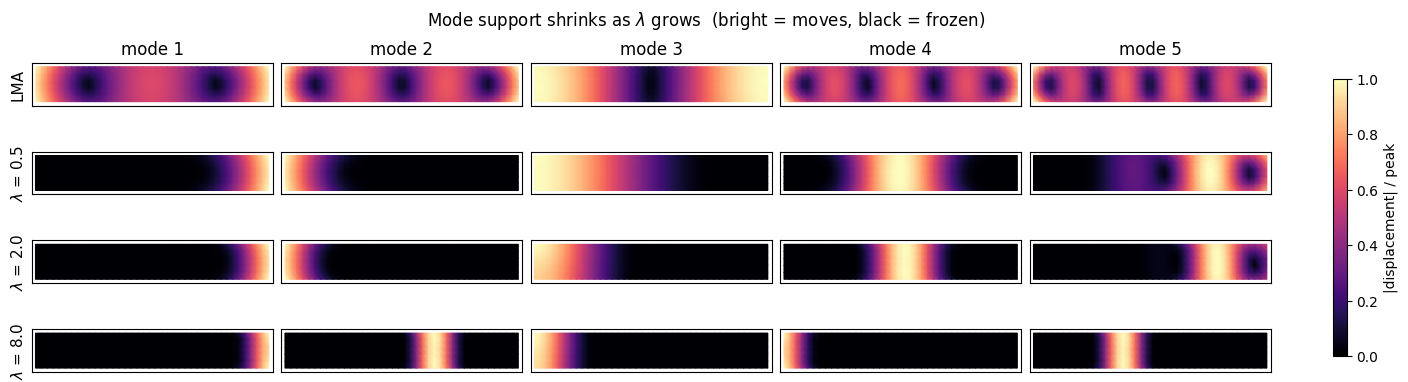
Each mode’s per-vertex displacement magnitude on the rest beam (normalized by its peak) shows its support at a glance: bright vertices move, black ones stay put. The top row is LMA, and each row below raises \(\lambda\). Mode order changes with \(\lambda\), so a column is not one mode followed down the rows. Still, the total bright area of a row shrinks as \(\lambda\) grows: the modes become sparser.
rows = {"LMA": B_lma, **{f"$\\lambda$ = {l}": B_iccm[l] for l in LAMBDAS}}
fig, axes = plt.subplots(len(rows), N_MODES, figsize=(14, 3.9), layout="constrained")
for r, (name, B) in enumerate(rows.items()):
    mag = mode_magnitude(B)
    for j in range(N_MODES):
        field = utils.plot_scalar_field(axes[r, j], X, T, mag[:, j] / mag[:, j].max(), cmap="magma",
                                        vmin=0, vmax=1, edges=False, colorbar=False,
                                        title=f"mode {j + 1}" if r == 0 else None)
        axes[r, j].set_xticks([])
        axes[r, j].set_yticks([])
    axes[r, 0].set_ylabel(name, fontsize=11)
fig.colorbar(field, ax=axes, shrink=0.8, label="|displacement| / peak")
fig.suptitle("Mode support shrinks as $\\lambda$ grows  (bright = moves, black = frozen)")
simkit.filesystem.save_figure(fig, os.path.join(RESULTS_DIR, "heatmaps.png"),
                              copy_to=os.path.join(MEDIA_DIR, "019_heatmaps.png"))
plt.show()
Quantifying sparsity#
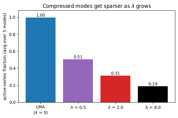
The active-vertex fraction, averaged over the five modes, falls steeply with \(\lambda\): LMA modes touch every vertex, and by \(\lambda = 8\) each mode moves under a fifth of the beam.
labels = ["LMA\n($\\lambda$ = 0)"] + [f"$\\lambda$ = {l}" for l in LAMBDAS]
fractions = [active_fraction(B_lma)] + [active_fraction(B_iccm[l]) for l in LAMBDAS]

fig, ax = plt.subplots(figsize=(6, 4))
ax.bar(labels, fractions, color=["#1f77b4", "#9467bd", "#d62728", "#000000"])
for i, v in enumerate(fractions):
    ax.text(i, v + 0.01, f"{v:.2f}", ha="center", fontsize=10)
ax.set_ylim(0, 1.08)
ax.set_ylabel(f"active-vertex fraction (avg over {N_MODES} modes)")
ax.set_title("Compressed modes get sparser as $\\lambda$ grows")
fig.tight_layout()
simkit.filesystem.save_figure(fig, os.path.join(RESULTS_DIR, "sparsity.png"),
                              copy_to=os.path.join(MEDIA_DIR, "019_sparsity.png"))
plt.show()
Did the solver lower its objective?#
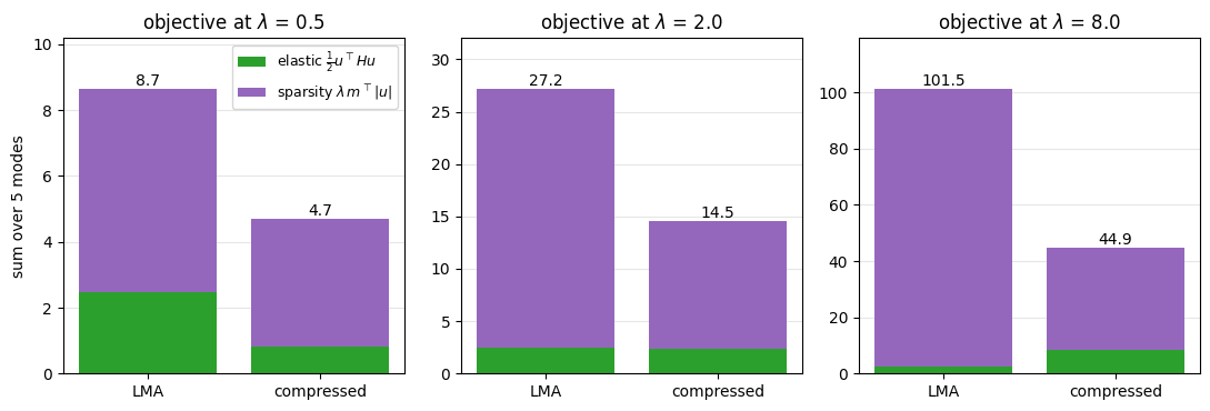
Both bases are \(M\)-normalized, so we can score each against the compressed objective of every \(\lambda\), split
into its two terms (the elastic part is beam_energy at \(X + u\), i.e. \(\tfrac12 u^\top H u\)). LMA modes are
elastically cheap but pay the sparsity term on every vertex; the compressed modes roughly halve the total.
Their elastic part grows with \(\lambda\) (at \(\lambda = 8\) they buy locality with stiffness). At \(\lambda = 0.5\)
it is even below LMA’s, since unlike the LMA deformation modes they are not \(M\)-orthogonal to the rigid
motions and can let a patch move almost rigidly.
fig, axes = plt.subplots(1, len(LAMBDAS), figsize=(11, 3.8))
for ax, l in zip(axes, LAMBDAS):
    mode_energy, mode_gradient, mode_hessian = compressed_mode_system(H, M, l)
    for i, (name, B) in enumerate([("LMA", B_lma), ("compressed", B_iccm[l])]):
        E_elastic = sum(beam_energy(x_rest + B[:, [j]]) for j in range(N_MODES))
        E_total = sum(mode_energy(B[:, [j]]) for j in range(N_MODES))
        E_sparse = E_total - E_elastic
        ax.bar(i, E_elastic, color="#2ca02c", label="elastic $\\frac{1}{2}u^\\top Hu$" if i == 0 else None)
        ax.bar(i, E_sparse, bottom=E_elastic, color="#9467bd",
               label="sparsity $\\lambda\\, m^\\top|u|$" if i == 0 else None)
        ax.text(i, E_total, f"{E_total:.1f}", ha="center", va="bottom", fontsize=10)
    ax.set_xticks([0, 1], ["LMA", "compressed"])
    ax.set_ylim(0, 1.12 * ax.get_ylim()[1])
    ax.set_title(f"objective at $\\lambda$ = {l}")
    ax.grid(True, axis="y", color="0.9")
    ax.set_axisbelow(True)
axes[0].set_ylabel(f"sum over {N_MODES} modes")
axes[0].legend(loc="upper right", fontsize=9)
fig.tight_layout()
simkit.filesystem.save_figure(fig, os.path.join(RESULTS_DIR, "objective.png"),
                              copy_to=os.path.join(MEDIA_DIR, "019_objective.png"))
plt.show()
Takeaways#
LMA modes are global. They diagonalize \(H\) against \(M\), and the low-frequency shapes span the whole body: great for spectral analysis, awkward for local editing.
An \(L_1\) penalty buys locality. Minimizing \(\tfrac12 u^\top H u + \lambda\, m^\top|u|\) (mass-normalized, deflated) keeps a mode smooth where it lives and exactly zero everywhere else.
One knob. \(\lambda\) slides from global LMA (\(\lambda \to 0\)) to tight local bumps (large \(\lambda\)), with nothing else touched.
simkit.eigs_iccmworks for any \((H, M)\) pair, giving a local basis for part-based deformation, sparse control and domain-decomposed reduced simulation, where a global basis couples everything to everything.