5 · Solving the Minimization: Newton vs. Gradient Descent#
Time to open the solver box. We pin a beam’s left edge, drag its whole right edge toward a target down and to the right, and drive the beam to equilibrium from rest with two methods that differ only in their search direction, gradient descent and Newton. Per iteration we track the energy, the gradient norm \(\lVert\nabla E\rVert\) and the Newton decrement \(\lambda = \sqrt{\nabla E^\top H^{-1}\nabla E}\).
Imports, and every tunable parameter of this notebook.
%matplotlib inline
import os
import numpy as np
import scipy as sp
import matplotlib.pyplot as plt
from matplotlib.colors import LogNorm
import igl
import simkit
import utils

NOTEBOOK = "005_numerical_solver"                                  # this file's name
RESULTS_DIR = utils.notebook_results_path(NOTEBOOK) # results/005_numerical_solver/
MEDIA_DIR = "media"                                                # tracked copies for the website
# mesh
NX, NY = 12, 4                          # grid vertices along x and y
WIDTH, HEIGHT = 2.0, 0.4                # beam size
# material: a soft beam
MATERIAL = "macklin-mueller-neo-hookean"   # simkit elastic model (the old utils "Neo-Hookean")
YM, PR = 0.5, 0.45                      # Young's modulus, Poisson ratio
# boundary conditions
K_PIN = 1e2                             # gentle pin spring on the left edge
K_HANDLE = 25.0                         # soft handle spring on the right edge
HANDLE_OFFSET = np.array([0.5, -0.7])   # handle targets = rest right edge + this offset
# solvers
MAX_ITERS = 60                          # iteration cap for both solvers
TOL = 1e-9                              # stop once the step ||alpha dx|| is smaller than this
# finite-difference check
FD_STEP = 1e-6                          # central-difference step
FD_NOISE = 0.05                         # std of the random perturbation of the rest state
SEED = 0                                # RNG seed for that perturbation
# visuals
LIMS = ((-1.2, 1.8), (-1.3, 0.6))       # plot window around the beam and its targets
FPS_NEWTON = 4                          # one frame per Newton iteration
FPS_GD = 10                             # one frame per gradient-descent iteration
PSI_RANGE = (1e-3, 3.0)                 # log color range of the energy-density plots
The beam#
A \(2\times0.4\) beam from libigl’s unit grid, with the constant operators the energy needs built
once: the deformation Jacobian \(J\) (each element’s \(F\) is a block of \(Jx\)), the per-element area
and the per-element Lamé parameters. The left-edge vertices are pinned in place and the right-edge
vertices form the handle, aimed at their rest positions shifted by HANDLE_OFFSET. The top panel
marks pins (blue), handle (orange) and targets (×). The bottom panel shows the per-element
area that weights each element’s energy; it is uniform here and sums to the beam’s area.
V, T = igl.triangulated_grid(NX, NY)                 # unit square, NX x NY vertices
X = (V - 0.5) * np.array([WIDTH, HEIGHT])            # centered WIDTH x HEIGHT beam
n, dim = X.shape
J = simkit.deformation_jacobian(X, T)                # per-element F = (J @ x).reshape(-1, dim, dim)
vol = simkit.volume(X, T)                            # per-element area
mu, lam = simkit.ympr_to_lame(YM, PR)
mu = np.full((len(T), 1), mu)                        # per-element Lame parameters
lam = np.full((len(T), 1), lam)

pin_idx = np.where(X[:, 0] <= X[:, 0].min() + 1e-6)[0]
handle_idx = np.where(X[:, 0] >= X[:, 0].max() - 1e-6)[0]
handle_targets = X[handle_idx] + HANDLE_OFFSET

fig, axes = plt.subplots(2, 1, figsize=(7, 6.5))
utils.plot_mesh(axes[0], X, T, pins=pin_idx, handles=handle_idx, lims=LIMS,
                title=f"rest beam: {n} vertices, {len(T)} triangles")
axes[0].scatter(*handle_targets.T, marker="x", s=60, linewidths=2, color="0.3", zorder=6,
                label="target")
axes[0].legend(loc="upper right", fontsize=8)
utils.plot_scalar_field(axes[1], X, T, vol, vmin=0.0, vmax=1.2 * vol.max(),
                        title="per-element area", label="area")
fig.tight_layout()
simkit.filesystem.save_figure(fig, os.path.join(RESULTS_DIR, "mesh.png"),
                              copy_to=os.path.join(MEDIA_DIR, "005_mesh.png"))
plt.show()
print(f"total area = {vol.sum():.4f}  (WIDTH * HEIGHT = {WIDTH * HEIGHT:.4f})")
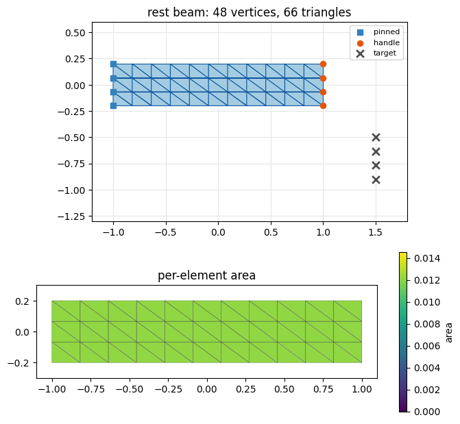
total area = 0.8000 (WIDTH * HEIGHT = 0.8000)
The objective#
Elastic energy plus a gentle pin spring and a soft handle spring. The handle spring is kept soft, with forces of the same magnitude as the elastic ones, so the problem is not horribly ill-conditioned. With a stiff handle, gradient descent just yanks the handle and leaves the rest of the beam untouched.
def beam_system(X, J, vol, mu, lam, pin_idx, pin_targets, handle_idx, handle_targets):
    """Neo-Hookean beam + soft pin + soft handle, in stacked vertex positions x."""
    n, dim = X.shape
    Q_pin, b_pin = simkit.dirichlet_penalty(pin_idx, pin_targets, n, K_PIN)
    Q_handle, b_handle = simkit.dirichlet_penalty(handle_idx, handle_targets, n, K_HANDLE)

    def energy_func(x):
        E_elastic = simkit.energies.elastic_energy_x(x.reshape(n, dim), J, mu, lam, vol, MATERIAL)
        E_pin = simkit.energies.quadratic_energy(x, Q_pin, b_pin)
        E_handle = simkit.energies.quadratic_energy(x, Q_handle, b_handle)
        E_total = E_elastic + E_pin + E_handle
        return E_total

    def gradient_func(x):
        g_elastic = simkit.energies.elastic_gradient_x(x.reshape(n, dim), J, mu, lam, vol, MATERIAL)
        g_pin = simkit.energies.quadratic_gradient(x, Q_pin, b_pin)
        g_handle = simkit.energies.quadratic_gradient(x, Q_handle, b_handle)
        g_total = g_elastic + g_pin + g_handle
        return g_total

    def hessian_func(x):
        H_elastic = simkit.energies.elastic_hessian_x(x.reshape(n, dim), J, mu, lam, vol, MATERIAL, psd=True)
        H_pin = simkit.energies.quadratic_hessian(Q_pin)
        H_handle = simkit.energies.quadratic_hessian(Q_handle)
        H_total = H_elastic + H_pin + H_handle
        return H_total

    return energy_func, gradient_func, hessian_func
The two solvers#
simkit’s newton_solver and gradient_descent run the same loop: evaluate \(g\) (and \(H\)), pick
\(\Delta x\), choose a step \(\alpha\) by backtracking line search (tutorial 6), set
\(x \leftarrow x + \alpha\Delta x\), and stop once \(\lVert\alpha\Delta x\rVert <\) TOL or after
MAX_ITERS steps. We run both from the rest state on the same objective with
return_info=True, which records every step \((\Delta x_k, \alpha_k)\), and then recompute both
first directions at \(x_0\) by hand to confirm that the direction is the only difference.
energy_func, gradient_func, hessian_func = beam_system(X, J, vol, mu, lam, pin_idx, X[pin_idx],
                                                       handle_idx, handle_targets)
x0 = X.reshape(-1, 1).copy()
_, newton_info = simkit.solvers.newton_solver(x0, energy_func, gradient_func, hessian_func,
                                              tolerance=TOL, max_iter=MAX_ITERS,
                                              do_line_search=True, return_info=True)
_, gd_info = simkit.solvers.gradient_descent(x0, energy_func, gradient_func,
                                             tolerance=TOL, max_iter=MAX_ITERS,
                                             do_line_search=True, return_info=True)

g0 = gradient_func(x0)
dx_gd = -g0                                                                         # -grad E
dx_newton = sp.sparse.linalg.spsolve(hessian_func(x0).tocsc(), -g0).reshape(-1, 1)  # -H^-1 grad E
cos_angle = (dx_gd.T @ dx_newton).item() / (np.linalg.norm(dx_gd) * np.linalg.norm(dx_newton))
print(f"first recorded step equals the hand-computed direction: "
      f"gradient descent {np.allclose(dx_gd, gd_info['dx'][0])}, "
      f"Newton {np.allclose(dx_newton, newton_info['dx'][0])}")
print(f"|dx_GD| = {np.linalg.norm(dx_gd):.1f}, |dx_Newton| = {np.linalg.norm(dx_newton):.1f}, "
      f"angle between them = {np.degrees(np.arccos(cos_angle)):.0f} deg")
first recorded step equals the hand-computed direction: gradient descent True, Newton True
|dx_GD| = 43.0, |dx_Newton| = 3.6, angle between them = 62 deg
Both recorded first steps are exactly \(-\nabla E\) and \(-H^{-1}\nabla E\), and already at rest they
disagree: the Newton step is about 12 times shorter and points 62° away from \(-\nabla E\). Next,
iterates rebuilds \(x_0, x_1, \dots\) from the recorded steps and solver_metrics measures each
one. It forms \(H\) at the gradient-descent iterates only to monitor \(\lambda\); gradient descent
itself never forms \(H\).
def iterates(x0, info):
    """x_0, x_1, ... rebuilt from the recorded steps x_{k+1} = x_k + alpha_k dx_k."""
    xs = [x0]
    for alpha, dx in zip(info["alphas"], info["dx"]):
        xs.append(xs[-1] + alpha * dx)
    return xs

def solver_metrics(xs):
    """Energy, gradient norm and Newton decrement sqrt(g^T H^-1 g) at every iterate."""
    energy, grad, decrement = [], [], []
    for x in xs:
        g = gradient_func(x)
        H_inv_g = sp.sparse.linalg.spsolve(hessian_func(x).tocsc(), g).reshape(-1, 1)
        energy.append(energy_func(x))
        grad.append(np.linalg.norm(g))
        decrement.append(np.sqrt(max((g.T @ H_inv_g).item(), 0.0)))
    return {"energy": energy, "grad": grad, "decrement": decrement}

newton_xs = iterates(x0, newton_info)
gd_xs = iterates(x0, gd_info)
newton_metrics = solver_metrics(newton_xs)
gd_metrics = solver_metrics(gd_xs)
for name, xs, m in [("Newton", newton_xs, newton_metrics), ("Gradient descent", gd_xs, gd_metrics)]:
    print(f"{name:17s}: {len(xs) - 1:2d} iters, final |grad| = {m['grad'][-1]:.2e}, "
          f"final E - E_Newton = {m['energy'][-1] - newton_metrics['energy'][-1]:.2e}, "
          f"final lambda = {m['decrement'][-1]:.2e}")
Newton           :  6 iters, final |grad| = 2.26e-14, final E - E_Newton = 0.00e+00, final lambda = 2.46e-15
Gradient descent : 60 iters, final |grad| = 6.09e-01, final E - E_Newton = 1.54e-01, final lambda = 5.08e-01
Newton reaches a round-off-level gradient in 6 iterations, while gradient descent uses all 60 and still sits 0.15 above Newton’s energy.
Checking the derivatives#
Both solvers trust gradient_func, and Newton also trusts hessian_func, so we check them against
central differences (simkit.gradient_cfd): the gradient at a randomly perturbed rest state, and
the Hessian there and at Newton’s equilibrium \(x^\star\). psd=True projects each element Hessian to
be positive semi-definite, so that \(-H^{-1}\nabla E\) is always a descent direction. The Hessian can
therefore match only where no projection is active.
rng = np.random.default_rng(SEED)
x_pert = x0 + FD_NOISE * rng.standard_normal(x0.shape)
x_star = newton_xs[-1]

g = gradient_func(x_pert)
g_fd = simkit.gradient_cfd(lambda y: np.array([energy_func(y.reshape(-1, 1))]), x_pert.ravel(), FD_STEP)
g_err = np.linalg.norm(g_fd.ravel() - g.ravel()) / np.linalg.norm(g)
print(f"gradient at perturbed rest: rel. error {g_err:.1e}")
for name, x in [("perturbed rest", x_pert), ("equilibrium x*", x_star)]:
    H = hessian_func(x).toarray()
    H_fd = simkit.gradient_cfd(lambda y: gradient_func(y.reshape(-1, 1)).ravel(), x.ravel(), FD_STEP)
    H_err = np.linalg.norm(H_fd - H) / np.linalg.norm(H)
    print(f"Hessian  at {name}: rel. error {H_err:.1e}")
gradient at perturbed rest: rel. error 2.6e-09
Hessian  at perturbed rest: rel. error 4.1e-02
Hessian  at equilibrium x*: rel. error 2.9e-11
The gradient matches to \(10^{-9}\), and the Hessian matches at \(x^\star\) but differs by 4% at the perturbed state, where the projection is active.
Convergence curves#
Energy gap to the optimum, gradient norm and Newton decrement per iteration, all on a log scale.
fig, _ = utils.convergence_plot({"Newton": newton_metrics, "Gradient Descent": gd_metrics},
                                title="Newton vs. Gradient Descent on the same problem")
simkit.filesystem.save_figure(fig, os.path.join(RESULTS_DIR, "convergence.png"),
                              copy_to=os.path.join(MEDIA_DIR, "005_convergence.png"))
plt.show()
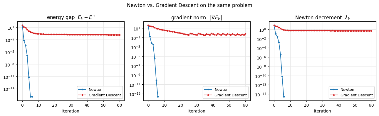
Newton’s curves drop steeply, with the number of correct digits roughly doubling per step at the end (quadratic convergence). Gradient descent flattens out after about 10 iterations, stalled by the ill-conditioned elastic Hessian. Its \(\lambda\) stays near 0.5, and since \(\lambda^2/2\) estimates \(E - E^\star\), that predicts a remaining gap of about 0.13, close to the true 0.15. The accepted line-search step \(\alpha_k\), plotted next, shows why gradient descent stalls.
fig, ax = plt.subplots(figsize=(6.5, 4))
for name, info in [("Newton", newton_info), ("Gradient Descent", gd_info)]:
    ax.semilogy(info["alphas"], "-o", ms=3, color=utils.SOLVER_COLORS[name], label=name)
ax.set_xlabel("iteration")
ax.set_ylabel(r"accepted step $\alpha_k$")
ax.set_title("line-search step size")
ax.grid(True, which="both", color="0.9", linewidth=0.7)
ax.legend(fontsize=9)
simkit.filesystem.save_figure(fig, os.path.join(RESULTS_DIR, "step_sizes.png"),
                              copy_to=os.path.join(MEDIA_DIR, "005_step_sizes.png"))
plt.show()
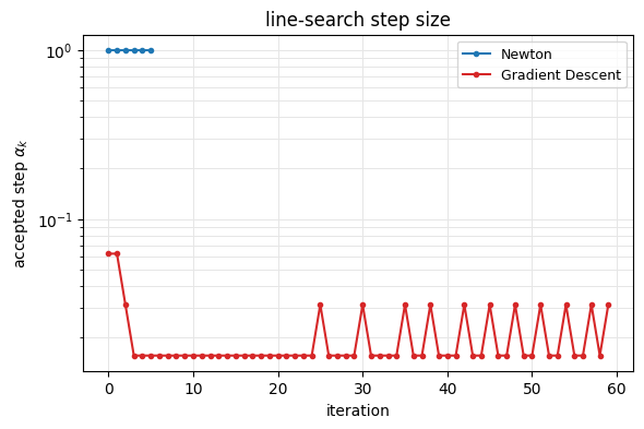
Newton takes the full step \(\alpha = 1\) every time, while along \(-\nabla E\) the stiff directions dominate, so only a tiny step lowers the energy (\(\alpha = 1/16\) for the first two steps, then mostly \(1/64\) with an occasional \(1/32\)).
Watching the beam converge (one frame per iteration)#
Newton first: after one step the whole beam is already bent into nearly its final shape.
fig, anim = utils.animate_mesh([x.reshape(n, dim) for x in newton_xs], T, lims=LIMS,
                               title="Newton's method", pin_pts=X[pin_idx],
                               handle_traj=[x.reshape(n, dim)[handle_idx] for x in newton_xs],
                               target_pts=[handle_targets] * len(newton_xs), fps=FPS_NEWTON)
video = simkit.filesystem.save_animation(anim, os.path.join(RESULTS_DIR, "newton.mp4"), fps=FPS_NEWTON,
                                         copy_to=os.path.join(MEDIA_DIR, "005_newton.mp4"))
plt.close(fig)
utils.embed_video(video)
Gradient descent: the handle reaches its target quickly, but the deformation only creeps back from the handle, leaving the left part of the beam nearly straight after 60 iterations.
fig, anim = utils.animate_mesh([x.reshape(n, dim) for x in gd_xs], T, lims=LIMS,
                               title="Gradient descent", pin_pts=X[pin_idx],
                               handle_traj=[x.reshape(n, dim)[handle_idx] for x in gd_xs],
                               target_pts=[handle_targets] * len(gd_xs), fps=FPS_GD)
video = simkit.filesystem.save_animation(anim, os.path.join(RESULTS_DIR, "gradient_descent.mp4"),
                                         fps=FPS_GD,
                                         copy_to=os.path.join(MEDIA_DIR, "005_gradient_descent.mp4"))
plt.close(fig)
utils.embed_video(video)
Where the energy sits#
The per-element energy density \(\psi(F)\) at both final states, with \(F\) from the same \(J\) and the same \(\mu, \lambda\) the energy uses, on one log color scale, and each vertex’s distance between the gradient-descent result and \(x^\star\).
F_newton = (J @ x_star).reshape(-1, dim, dim)       # per-element F, as in the energy
F_gd = (J @ gd_xs[-1]).reshape(-1, dim, dim)
psi_newton = simkit.energies.elastic_energy_element_F(F_newton, mu, lam, MATERIAL).ravel()
psi_gd = simkit.energies.elastic_energy_element_F(F_gd, mu, lam, MATERIAL).ravel()
gd_error = np.linalg.norm((gd_xs[-1] - x_star).reshape(n, dim), axis=1)

lims = utils.auto_limits([x_star.reshape(n, dim), gd_xs[-1].reshape(n, dim)], pad=0.1)
fig, axes = plt.subplots(3, 1, figsize=(7.5, 8.5))
utils.plot_scalar_field(axes[0], x_star.reshape(n, dim), T, psi_newton, lims=lims, cmap="magma",
                        norm=LogNorm(*PSI_RANGE), title=r"Newton: energy density $\psi$", label=r"$\psi$")
utils.plot_scalar_field(axes[1], gd_xs[-1].reshape(n, dim), T, psi_gd, lims=lims, cmap="magma",
                        norm=LogNorm(*PSI_RANGE), title=r"gradient descent: energy density $\psi$",
                        label=r"$\psi$")
utils.plot_scalar_field(axes[2], gd_xs[-1].reshape(n, dim), T, gd_error, lims=lims,
                        title=r"gradient descent: distance to Newton's solution",
                        label=r"$\|x_i - x_i^\star\|$")
fig.tight_layout()
simkit.filesystem.save_figure(fig, os.path.join(RESULTS_DIR, "energy_density.png"),
                              copy_to=os.path.join(MEDIA_DIR, "005_energy_density.png"))
plt.show()
print(f"max psi: Newton {psi_newton.max():.3f}, gradient descent {psi_gd.max():.3f}; "
      f"max vertex error of gradient descent {gd_error.max():.3f}")
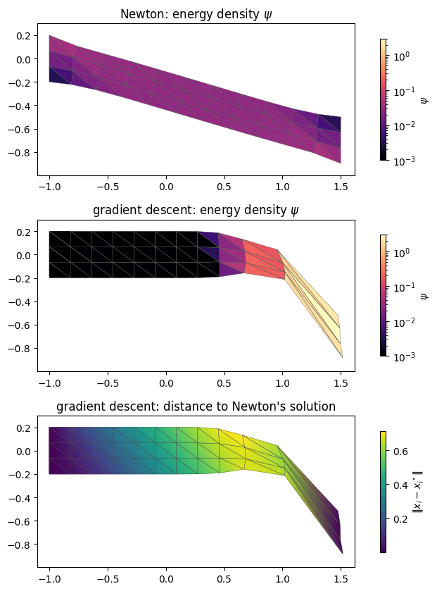
max psi: Newton 0.040, gradient descent 2.952; max vertex error of gradient descent 0.715
Newton spreads a gentle bend along the whole beam (peak \(\psi = 0.04\)), while gradient descent packs the strain into a kink by the handle (peak \(\psi = 2.95\)), leaves the pinned half unstrained, and is off by up to 0.72 just before the kink.
Takeaways#
Newton uses curvature and converges quadratically, which is ideal for stiff elasticity.
Gradient descent ignores curvature, gets tiny line-search steps, and stalls.
The Newton decrement is a clean, scale-aware stopping measure.
The Newton step length still needs care, which is the subject of tutorial 6.