7 · Time Integration: Forward Euler, Backward Euler, BDF2#
To animate motion we march Newton’s law \(M\ddot x = -\nabla V(x)\) forward in time with a step \(h\). We compare three integrators on the same pinned cantilever beam: Forward Euler (explicit, order 1, cheap but explodes unless \(h\) is tiny), Backward Euler (implicit, order 1, stable but damps) and BDF2 (implicit, order 2, barely damps). Each implicit step minimizes the potential plus an inertia term that pulls \(x\) toward where momentum alone would carry it (\(\tilde x\)); the two implicit schemes differ only in \(\tilde x\) and the weight \(c\):
Imports, and every tunable parameter of this notebook.
%matplotlib inline
import os
import numpy as np
import scipy as sp
import matplotlib.pyplot as plt
import igl
import simkit
import utils

NOTEBOOK = "007_time_integration"                                  # this file's name
RESULTS_DIR = utils.notebook_results_path(NOTEBOOK)                # results/007_time_integration/
MEDIA_DIR = "media"                                                # tracked copies for the website
# mesh
NX, NY = 14, 4                      # grid resolution (vertices along x, y)
WIDTH, HEIGHT = 2.0, 0.3            # beam size
# material and loads
MATERIAL = "macklin-mueller-neo-hookean"   # elastic energy model passed to simkit.energies.elastic_*_x
YM, PR = 500.0, 0.4                 # Young's modulus, Poisson ratio
RHO = 1.0                           # density
GRAVITY = -9.8                      # vertical gravitational acceleration
K_PIN = 1e7                         # soft-pin stiffness on the left edge
# implicit solves
NEWTON_ITERS = 30                   # max Newton iterations per implicit step
NEWTON_TOL = 1e-6                   # Newton stops when the step is shorter than this
# validation
H_CHECK = 0.01                      # timestep of the sanity checks
FD_STEP = 1e-6                      # central-difference step of the gradient check
FD_NOISE = 0.01                     # size of the random pose / velocity perturbations of the checks
SEED = 0                            # random seed of that perturbation
# order of accuracy
T_ORDER = 0.5                       # final time of the accuracy study
H_REF = 0.0003125                   # fine BDF2 reference timestep
H_ORDER = [0.02, 0.01, 0.005, 0.0025]   # timesteps whose error is measured
H_ERROR_FIELD = 0.01                # timestep whose per-vertex error is drawn
# forward vs backward Euler
H_BLOW = 0.008                      # timestep of the explicit/implicit race
H_FE_SMALL = 0.0002                 # a timestep small enough for Forward Euler to survive T_BLOW
T_BLOW = 0.3                        # its duration
BLOW_LIMIT = 1e3                    # a coordinate beyond this counts as "exploded"
N_FRAMES_BLOW, FPS_BLOW = 40, 20    # its video
# numerical damping
T_DAMP = 3.0                        # duration of the damping study
DTS = [0.001, 0.01, 0.1]            # timesteps compared
N_FRAMES_DAMP, FPS_DAMP = 60, 30    # its videos
The beam#
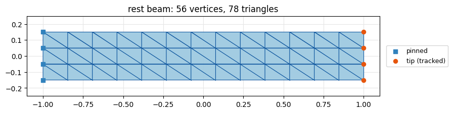
A \(2 \times 0.3\) grid from libigl, with its left edge pinned. We also track the right-edge (“tip”) vertices to measure the swing later. Blue squares mark the pinned vertices, orange dots the tip.
V_grid, T = igl.triangulated_grid(NX, NY)                 # unit square, NX x NY vertices
X = (V_grid - 0.5) * np.array([WIDTH, HEIGHT])           # centered WIDTH x HEIGHT beam
n, dim = X.shape
pin_idx = np.where(X[:, 0] <= X[:, 0].min() + 1e-6)[0]
tip_idx = np.where(X[:, 0] >= X[:, 0].max() - 1e-6)[0]
x_rest = X.reshape(-1, 1)

fig, ax = plt.subplots(figsize=(9, 2.4))
utils.plot_mesh(ax, X, T, pins=pin_idx, title=f"rest beam: {n} vertices, {len(T)} triangles")
ax.scatter(X[tip_idx, 0], X[tip_idx, 1], s=34, color=utils.HANDLE_C, zorder=5, label="tip (tracked)")
ax.legend(loc="center left", bbox_to_anchor=(1.01, 0.5), fontsize=9)
simkit.filesystem.save_figure(fig, os.path.join(RESULTS_DIR, "mesh.png"),
                              copy_to=os.path.join(MEDIA_DIR, "007_mesh.png"))
plt.show()
Constant operators#
Everything that does not change during a simulation is built once from simkit: the deformation
Jacobian J, triangle areas vol, Lamé parameters, the (lumped, diagonal) mass matrix M, the gravity
force f_g, and the soft-pin penalty (Q_pin, b_pin). The scalar fields the dynamics rely on are
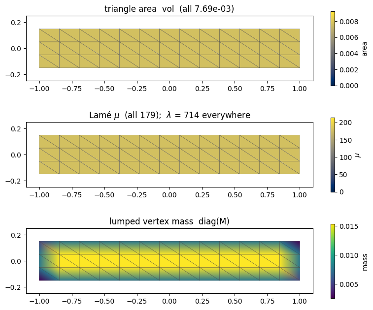
drawn below: every triangle of this regular grid has the same area and the same Lamé parameters
\(\mu, \lambda\), and each vertex’s mass is a share of its neighbouring triangles’ area, so boundary
vertices carry half the interior mass and the corners the least (darker colours).
J = simkit.deformation_jacobian(X, T)
vol = simkit.volume(X, T)
mu_value, lam_value = simkit.ympr_to_lame(YM, PR)
mu = np.full((len(T), 1), mu_value)
lam = np.full((len(T), 1), lam_value)
M_vertex = simkit.massmatrix(X, T, rho=RHO)                 # (n, n) lumped mass
M = sp.sparse.kron(M_vertex, sp.sparse.eye(dim)).tocsc()     # (n*dim, n*dim)
f_g = simkit.gravity_force(X, T, a=GRAVITY, rho=RHO).reshape(-1, 1)
Q_pin, b_pin = simkit.dirichlet_penalty(pin_idx, X[pin_idx], n, K_PIN)

fig, axes = plt.subplots(3, 1, figsize=(8, 6.6))
utils.plot_scalar_field(axes[0], X, T, vol, title=f"triangle area  vol  (all {vol.mean():.2e})",
                        cmap="cividis", vmin=0.0, vmax=1.2 * vol.max(), label="area")
utils.plot_scalar_field(axes[1], X, T, mu, cmap="cividis", vmin=0.0, vmax=1.2 * mu_value, label=r"$\mu$",
                        title=rf"Lamé $\mu$  (all {mu_value:.0f});  $\lambda$ = {lam_value:.0f} everywhere")
utils.plot_scalar_field(axes[2], X, T, M_vertex.diagonal(), title="lumped vertex mass  diag(M)",
                        cmap="viridis", label="mass")
fig.tight_layout()
simkit.filesystem.save_figure(fig, os.path.join(RESULTS_DIR, "area_mass.png"),
                              copy_to=os.path.join(MEDIA_DIR, "007_area_mass.png"))
plt.show()
The potential \(V(x)\)#
beam_potential_system returns the static potential: elastic energy, the pinned left edge and gravity,
one term per line. Gravity is linear in \(x\), so it has no Hessian term. Forward Euler only needs its
gradient (the force is \(-\nabla V\)).
def beam_potential_system():
    """Potential V(x) of the beam: elastic + soft pin + gravity (no inertia)."""

    def energy_func(x):
        E_elastic = simkit.energies.elastic_energy_x(x.reshape(n, dim), J, mu, lam, vol, MATERIAL)
        E_pin = simkit.energies.quadratic_energy(x, Q_pin, b_pin)
        E_gravity = -(f_g.T @ x).item()
        E_total = E_elastic + E_pin + E_gravity
        return E_total

    def gradient_func(x):
        g_elastic = simkit.energies.elastic_gradient_x(x.reshape(n, dim), J, mu, lam, vol, MATERIAL)
        g_pin = simkit.energies.quadratic_gradient(x, Q_pin, b_pin)
        g_gravity = -f_g
        g_total = g_elastic + g_pin + g_gravity
        return g_total

    def hessian_func(x):
        H_elastic = simkit.energies.elastic_hessian_x(x.reshape(n, dim), J, mu, lam, vol, MATERIAL, psd=True)
        H_pin = simkit.energies.quadratic_hessian(Q_pin)
        H_total = H_elastic + H_pin
        return H_total

    return energy_func, gradient_func, hessian_func
One implicit step#
implicit_step_system(x_tilde, c, h) is the incremental potential minimized by every implicit step: the
potential plus the inertia term \(\tfrac{c}{2h^2}\lVert x-\tilde x\rVert_M^2\)
(simkit.energies.kinetic_energy and friends, applied to \(d = x - \tilde x\)). It is rebuilt at every
step with that step’s target.
def implicit_step_system(x_tilde, c, h):
    """Incremental potential of one implicit step: V(x) + c / (2 h^2) ||x - x_tilde||_M^2."""
    V_energy, V_gradient, V_hessian = beam_potential_system()

    def energy_func(x):
        E_potential = V_energy(x)
        E_inertia = simkit.energies.kinetic_energy(x - x_tilde, M, h, c)
        E_total = E_potential + E_inertia
        return E_total

    def gradient_func(x):
        g_potential = V_gradient(x)
        g_inertia = simkit.energies.kinetic_gradient(x - x_tilde, M, h, c)
        g_total = g_potential + g_inertia
        return g_total

    def hessian_func(x):
        H_potential = V_hessian(x)
        H_inertia = simkit.energies.kinetic_hessian(M, h, c)
        H_total = H_potential + H_inertia
        return H_total

    return energy_func, gradient_func, hessian_func
The three steppers#
Each maps the state (positions \(x_n\), velocities \(v_n\)) to the next one. Only the target \(\tilde x\), the weight \(c\) and the velocity update differ:
Forward Euler: \(x_{n+1} = x_n + h v_n\), \(\;v_{n+1} = v_n - h M^{-1}\nabla V(x_n)\) (
simkit.integrators.forward_euler, lumped mass, no solve). Pins are clamped afterwards.Backward Euler: \(c = 1\), \(\;\tilde x = x_n + h v_n\), \(\;v_{n+1} = (x_{n+1} - x_n)/h\).
BDF2: \(c = \tfrac94\), \(\;\tilde x = \tfrac43 x_n - \tfrac13 x_{n-1} + \tfrac{8h}{9} v_n - \tfrac{2h}{9} v_{n-1}\), \(\;v_{n+1} = (3x_{n+1} - 4x_n + x_{n-1})/(2h)\).
pin_dofs = (pin_idx[:, None] * dim + np.arange(dim)).ravel()

def forward_euler_step(x, v, h):
    """Explicit step: read the force at x_n, no solve."""
    V_energy, V_gradient, V_hessian = beam_potential_system()
    x_next, v_next = simkit.integrators.forward_euler(x, v, V_gradient, M, h)
    x_next[pin_dofs] = x_rest[pin_dofs]                      # hard-clamp the pins
    v_next[pin_dofs] = 0.0
    return x_next, v_next

def backward_euler_step(x, v, h):
    """Implicit step with c = 1 and target x_n + h v_n."""
    x_tilde = x + h * v
    energy_func, gradient_func, hessian_func = implicit_step_system(x_tilde, 1.0, h)
    x_next = simkit.solvers.newton_solver(x_tilde, energy_func, gradient_func, hessian_func,
                                          tolerance=NEWTON_TOL, max_iter=NEWTON_ITERS, do_line_search=True)
    v_next = (x_next - x) / h
    return x_next, v_next

def bdf2_step(x, v, x_prev, v_prev, h):
    """Implicit step with c = 9/4 and the second-order BDF2 target."""
    x_tilde = (4 / 3) * x - (1 / 3) * x_prev + (8 * h / 9) * v - (2 * h / 9) * v_prev
    energy_func, gradient_func, hessian_func = implicit_step_system(x_tilde, 9 / 4, h)
    x_next = simkit.solvers.newton_solver(x_tilde, energy_func, gradient_func, hessian_func,
                                          tolerance=NEWTON_TOL, max_iter=NEWTON_ITERS, do_line_search=True)
    v_next = (3 * x_next - 4 * x + x_prev) / (2 * h)
    return x_next, v_next
Sanity checks#
Three cheap checks before simulating: the step gradient matches a central finite difference
(simkit.gradient_cfd) at a random pose; our Backward Euler step from a random velocity matches the
library’s simkit.integrators.backward_euler (same Newton solve); and Newton converges on the first
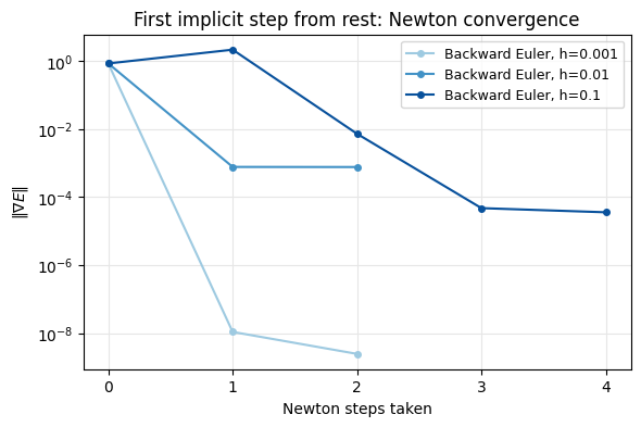
step from rest. Expect a gradient error near \(10^{-7}\) and a difference at rounding level. The plot shows
\(\lVert\nabla E\rVert\) after each Newton step; Newton stops once its step is shorter than NEWTON_TOL.
At \(h = 0.001\) and \(0.1\) the gradient drops by 8 and 4 orders of magnitude. At \(h = 0.01\) the line search
stalls after one step at \(\approx 8\cdot10^{-4}\) (the remaining decrease is below the rounding error of
the total energy), still 1000 times below the start and ample for one timestep.
rng = np.random.default_rng(SEED)
x_test = x_rest + FD_NOISE * rng.standard_normal(x_rest.shape)
energy_func, gradient_func, hessian_func = implicit_step_system(x_rest, 1.0, H_CHECK)
g_fd = simkit.gradient_cfd(lambda y: np.array(energy_func(y.reshape(-1, 1))), x_test.ravel(), FD_STEP)
g_an = gradient_func(x_test).ravel()
print(f"gradient check: relative error {np.linalg.norm(g_fd - g_an) / np.linalg.norm(g_an):.2e}")

v_test = FD_NOISE * rng.standard_normal(x_rest.shape)
x_ours, _ = backward_euler_step(x_rest, v_test, H_CHECK)
V_energy, V_gradient, V_hessian = beam_potential_system()
x_lib = simkit.integrators.backward_euler(x_rest, x_rest - H_CHECK * v_test, V_energy, V_gradient,
                                          V_hessian, M, H_CHECK, tolerance=NEWTON_TOL,
                                          max_iter=NEWTON_ITERS, do_line_search=True)
print(f"our BE step vs simkit.integrators.backward_euler: max difference {np.abs(x_ours - x_lib).max():.1e} "
      f"(the step itself moves vertices by up to {np.abs(x_ours - x_rest).max():.1e})")

fig, ax = plt.subplots(figsize=(6.5, 4))
for h, col in zip(DTS, ["#9ecae1", "#4292c6", "#08519c"]):
    energy_func, gradient_func, hessian_func = implicit_step_system(x_rest, 1.0, h)
    x_final, info = simkit.solvers.newton_solver(x_rest.copy(), energy_func, gradient_func, hessian_func,
                                                 tolerance=NEWTON_TOL, max_iter=NEWTON_ITERS,
                                                 do_line_search=True, return_info=True)
    g_norms = [np.linalg.norm(g) for g in info["g"]] + [np.linalg.norm(gradient_func(x_final))]
    ax.semilogy(g_norms, "-o", ms=4, color=col, label=f"Backward Euler, h={h}")
ax.set_xlabel("Newton steps taken"); ax.set_ylabel(r"$\|\nabla E\|$")
ax.xaxis.set_major_locator(plt.MaxNLocator(integer=True))
ax.set_title("First implicit step from rest: Newton convergence")
ax.grid(True, which="both", color="0.9"); ax.legend(fontsize=9)
simkit.filesystem.save_figure(fig, os.path.join(RESULTS_DIR, "newton_convergence.png"),
                              copy_to=os.path.join(MEDIA_DIR, "007_newton_convergence.png"))
plt.show()
gradient check: relative error 6.45e-08
our BE step vs simkit.integrators.backward_euler: max difference 1.1e-16 (the step itself moves vertices by up to 1.0e-03)
A driver that records every step#
simulate releases the beam from rest and takes exactly round(T/h) steps, so every timestep ends
at the same final time. It records all positions and velocities; BDF2 needs one step of history, so its
first step is a Backward Euler step. A run that blows up (non-finite, or beyond BLOW_LIMIT) stops early.
A short recorded BDF2 run then cross-checks bdf2_step against simkit.integrators.bdf2, which rebuilds
both velocities from the last four positions; the two should agree to rounding.
def simulate(scheme, h, T_total):
    """Integrate from rest with `scheme`; return times (K,), positions and velocities (K, n*dim)."""
    x, v = x_rest.copy(), np.zeros_like(x_rest)
    x_prev, v_prev = x, v
    xs, vs = [x], [v]
    for k in range(int(round(T_total / h))):
        if scheme == "Forward Euler":
            x_next, v_next = forward_euler_step(x, v, h)
        elif scheme == "Backward Euler" or k == 0:           # BDF2 bootstraps with one BE step
            x_next, v_next = backward_euler_step(x, v, h)
        else:
            x_next, v_next = bdf2_step(x, v, x_prev, v_prev, h)
        x_prev, v_prev, x, v = x, v, x_next, v_next
        xs.append(x); vs.append(v)
        if not np.isfinite(x).all() or np.abs(x).max() > BLOW_LIMIT:
            break
    ts = h * np.arange(len(xs))
    return ts, np.hstack(xs).T, np.hstack(vs).T

_, xs_check, vs_check = simulate("BDF2", H_CHECK, 4 * H_CHECK)       # states x_0 .. x_4
x_hist = [x.reshape(-1, 1) for x in xs_check[::-1]]                   # x_4, x_3, x_2, x_1, x_0
v_hist = [v.reshape(-1, 1) for v in vs_check[::-1]]
x_ours, _ = bdf2_step(x_hist[0], v_hist[0], x_hist[1], v_hist[1], H_CHECK)
V_energy, V_gradient, V_hessian = beam_potential_system()
x_lib = simkit.integrators.bdf2(x_hist[0], x_hist[1], x_hist[2], x_hist[3], V_energy, V_gradient, V_hessian,
                                M, H_CHECK, tolerance=NEWTON_TOL, max_iter=NEWTON_ITERS, do_line_search=True)
print(f"our BDF2 step vs simkit.integrators.bdf2: max difference {np.abs(x_ours - x_lib).max():.1e} "
      f"(the step itself moves vertices by up to {np.abs(x_ours - x_hist[0]).max():.1e})")
our BDF2 step vs simkit.integrators.bdf2: max difference 0.0e+00 (the step itself moves vertices by up to 4.5e-03)
Order of accuracy, measured on our beam#
We run the beam to \(T = 0.5\) at four timesteps and compare the final pose with a fine-timestep BDF2 reference on the same mesh. On a log-log plot an order-\(p\) method is a line of slope \(p\). Forward Euler is left out: it needs a far smaller \(h\) just to stay stable, as we’ll see next.
_, xs_ref, _ = simulate("BDF2", H_REF, T_ORDER)
x_ref = xs_ref[-1]
final = {(scheme, h): simulate(scheme, h, T_ORDER)[1][-1]
         for scheme in ["Backward Euler", "BDF2"] for h in H_ORDER}
errors = {scheme: np.array([np.linalg.norm(final[scheme, h] - x_ref) for h in H_ORDER])
          for scheme in ["Backward Euler", "BDF2"]}
for scheme, e in errors.items():
    fitted = np.polyfit(np.log(H_ORDER), np.log(e), 1)[0]
    last_pair = np.log(e[-2] / e[-1]) / np.log(H_ORDER[-2] / H_ORDER[-1])
    print(f"{scheme:16s} errors {np.array2string(e, precision=4)}   fitted order {fitted:.2f}   "
          f"slope between the two smallest h {last_pair:.2f}")

fig, ax = utils.loglog_plot(H_ORDER, errors, xlabel="timestep  h", ylabel="error vs fine reference",
                            colors=utils.INTEGRATOR_COLORS, ref_slopes={"O(h)": 1, "O(h^2)": 2},
                            title="Order of accuracy on the beam")
simkit.filesystem.save_figure(fig, os.path.join(RESULTS_DIR, "order_of_accuracy.png"),
                              copy_to=os.path.join(MEDIA_DIR, "007_order_of_accuracy.png"))
plt.show()
Backward Euler   errors [0.0985 0.0657 0.0399 0.0228]   fitted order 0.70   slope between the two smallest h 0.81
BDF2             errors [0.041  0.0144 0.0044 0.0011]   fitted order 1.72   slope between the two smallest h 1.95
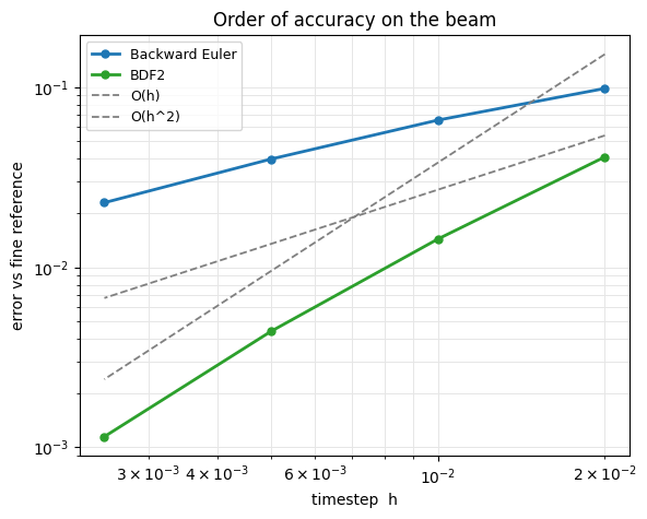
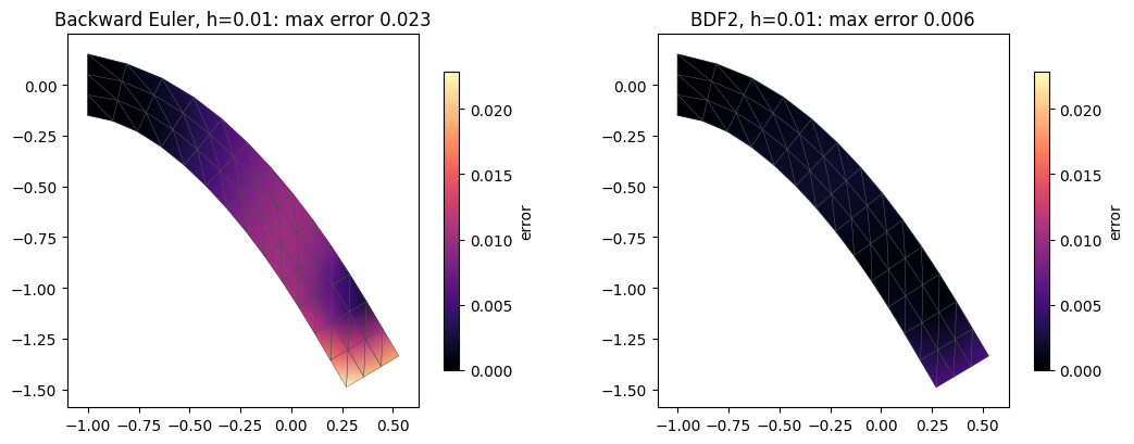
BDF2 is both more accurate and steeper. The fitted slopes (0.70, 1.72) sit below 1 and 2 because the largest timesteps are not yet asymptotic; between the two smallest they are 0.81 and 1.95. Where on the beam does the error live? Below is the per-vertex error \(\lVert x_i - x_i^{\text{ref}}\rVert\) at \(h = 0.01\), on the reference pose with a shared color scale: it is largest near the free tip, and BDF2’s is about four times smaller.
X_ref = x_ref.reshape(n, dim)
err_fields = {scheme: np.linalg.norm((final[scheme, H_ERROR_FIELD] - x_ref).reshape(n, dim), axis=1)
              for scheme in ["Backward Euler", "BDF2"]}
vmax = max(e.max() for e in err_fields.values())
fig, axes = plt.subplots(1, 2, figsize=(11, 4.2))
for ax, (scheme, e) in zip(axes, err_fields.items()):
    utils.plot_scalar_field(ax, X_ref, T, e, vmin=0.0, vmax=vmax, cmap="magma", label="error",
                            title=f"{scheme}, h={H_ERROR_FIELD}: max error {e.max():.3f}")
fig.tight_layout()
simkit.filesystem.save_figure(fig, os.path.join(RESULTS_DIR, "error_field.png"),
                              copy_to=os.path.join(MEDIA_DIR, "007_error_field.png"))
plt.show()
Forward Euler explodes; Backward Euler doesn’t#
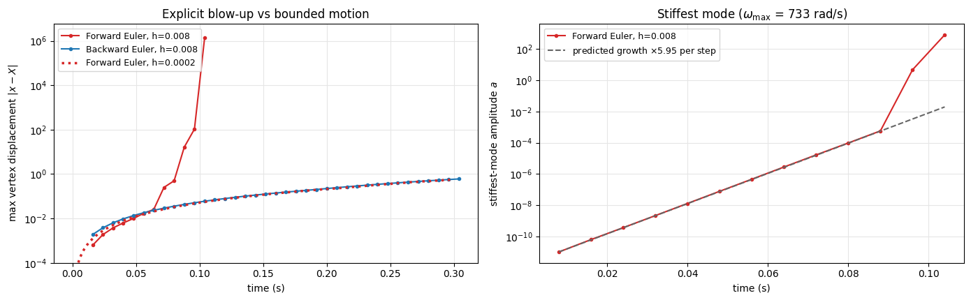
On a vibration mode of frequency \(\omega\), one Forward Euler step multiplies the amplitude by \(\sqrt{1 + \omega^2 h^2} > 1\), so the stiffest mode (\(\omega_{\max}\) of \(K u = \omega^2 M u\) at rest) grows fastest. We compute it and run both integrators at \(h = 0.008\). Left, the largest vertex displacement: Forward Euler follows Backward Euler while its unstable stiff modes are still tiny, then shoots up from \(t \approx 0.07\) s and leaves the scene after 13 steps. It survives the same 0.3 s only at \(h = 0.0002\) (dotted, on top of Backward Euler), a timestep 40 times smaller. Right, the amplitude \(a = \sqrt{q^2 + (\dot q/\omega_{\max})^2}\) of the stiffest mode \(u_{\max}\) itself, with \(q = u_{\max}^\top M (x - X)\): it grows at the predicted rate from the very first step.
free = np.setdiff1d(np.arange(n * dim), pin_dofs)
M_free = M[free][:, free]
K_rest = simkit.energies.elastic_hessian_x(X, J, mu, lam, vol, MATERIAL, psd=True)[free][:, free]
omega_sq, U = sp.linalg.eigh(K_rest.toarray(), M_free.toarray())      # K u = omega^2 M u, M-orthonormal u
omega_max, u_max = np.sqrt(omega_sq[-1]), U[:, -1]
growth = np.sqrt(1 + (omega_max * H_BLOW) ** 2)
print(f"omega_max = {omega_max:.0f} rad/s  ->  Forward Euler amplifies it x{growth:.2f} per step at h={H_BLOW}")

runs_blow = {scheme: simulate(scheme, H_BLOW, T_BLOW) for scheme in ["Forward Euler", "Backward Euler"]}
ts_small, xs_small, _ = simulate("Forward Euler", H_FE_SMALL, T_BLOW)
ts_fe, xs_fe, vs_fe = runs_blow["Forward Euler"]
q = np.array([u_max @ (M_free @ (x - x_rest.ravel())[free]) for x in xs_fe])    # stiffest-mode coordinate
q_dot = np.array([u_max @ (M_free @ v[free]) for v in vs_fe])                   # and its velocity
amp = np.hypot(q, q_dot / omega_max)
print(f"measured: the stiffest mode grows x{np.median(amp[2:] / amp[1:-1]):.2f} per step (median), "
      f"FE leaves the scene after {len(ts_fe) - 1} steps")

fig, axes = plt.subplots(1, 2, figsize=(14, 4.4))
ax = axes[0]
for scheme, (ts, xs, _) in runs_blow.items():
    disp = np.abs(xs - x_rest.ravel()).max(axis=1)
    ax.semilogy(ts[2:], disp[2:], "-o", ms=3, color=utils.INTEGRATOR_COLORS[scheme], label=f"{scheme}, h={H_BLOW}")
disp_small = np.abs(xs_small - x_rest.ravel()).max(axis=1)
ax.semilogy(ts_small[2:], disp_small[2:], ":", lw=2.5, color=utils.INTEGRATOR_COLORS["Forward Euler"],
            zorder=4, label=f"Forward Euler, h={H_FE_SMALL}")
ax.set_xlabel("time (s)"); ax.set_ylabel(r"max vertex displacement $|x - X|$")
ax.set_title("Explicit blow-up vs bounded motion"); ax.set_ylim(bottom=1e-4)
ax.grid(True, which="both", color="0.9"); ax.legend(fontsize=9, loc="upper left")
ax = axes[1]
k = np.arange(1, len(ts_fe))
ax.semilogy(ts_fe[k], amp[k], "-o", ms=3, color=utils.INTEGRATOR_COLORS["Forward Euler"],
            label=f"Forward Euler, h={H_BLOW}")
ax.semilogy(ts_fe[k], amp[1] * growth ** (k - 1), "--", color="0.4",
            label=rf"predicted growth $\times{growth:.2f}$ per step")
ax.set_xlabel("time (s)"); ax.set_ylabel(r"stiffest-mode amplitude $a$")
ax.set_title(rf"Stiffest mode ($\omega_{{\max}}$ = {omega_max:.0f} rad/s)")
ax.grid(True, which="both", color="0.9"); ax.legend(fontsize=9, loc="upper left")
fig.tight_layout()
simkit.filesystem.save_figure(fig, os.path.join(RESULTS_DIR, "fe_growth.png"),
                              copy_to=os.path.join(MEDIA_DIR, "007_fe_growth.png"))
plt.show()
omega_max = 733 rad/s  ->  Forward Euler amplifies it x5.95 per step at h=0.008
measured: the stiffest mode grows x5.98 per step (median), FE leaves the scene after 13 steps
The same two runs side by side: Forward Euler flies apart after about 0.1 s, while Backward Euler calmly sags under gravity. This is why stiff elasticity is integrated implicitly.
sample_blow = np.linspace(0, T_BLOW, N_FRAMES_BLOW)
panels = [{"states": utils.states_at_times(ts, xs.reshape(-1, n, dim), sample_blow), "T": T,
           "title": f"{scheme}  h={H_BLOW}" + ("  (EXPLODES)" if scheme == "Forward Euler" else "  (stable)")}
          for scheme, (ts, xs, _) in runs_blow.items()]
lims_blow = utils.auto_limits([runs_blow["Backward Euler"][1].reshape(-1, dim)], pad=0.3)   # frame the stable run
fig, anim = utils.animate_meshes_grid(panels, lims=lims_blow, fps=FPS_BLOW,
                                      suptitle="Same timestep: explicit blows up, implicit is fine")
video = simkit.filesystem.save_animation(anim, os.path.join(RESULTS_DIR, "fe_vs_be.mp4"), fps=FPS_BLOW,
                                         copy_to=os.path.join(MEDIA_DIR, "007_fe_vs_be.mp4"))
plt.close(fig)
utils.embed_video(video)
Numerical damping: the timestep changes perceived stiffness#
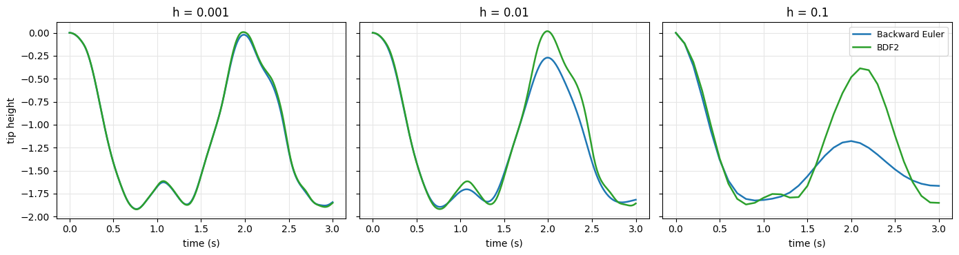
Release the beam under gravity and step Backward Euler for 3 s at \(h\) = 0.001, 0.01 and 0.1. The physics is identical, yet the larger the step, the more artificial damping: the swing dies out faster and the material looks stiffer. The cell simulates BDF2 at the same timesteps too, for the next sections.
sample_damp = np.linspace(0, T_DAMP, N_FRAMES_DAMP)
runs = {(scheme, h): simulate(scheme, h, T_DAMP) for scheme in ["Backward Euler", "BDF2"] for h in DTS}
lims_damp = utils.auto_limits([xs.reshape(-1, dim) for _, xs, _ in runs.values()], pad=0.15)

panels = [{"states": utils.states_at_times(runs["Backward Euler", h][0],
                                           runs["Backward Euler", h][1].reshape(-1, n, dim), sample_damp),
           "T": T, "title": f"Backward Euler  h={h}"} for h in DTS]
fig, anim = utils.animate_meshes_grid(panels, lims=lims_damp, fps=FPS_DAMP,
                                      suptitle="Backward Euler: bigger timestep -> more numerical damping")
video = simkit.filesystem.save_animation(anim, os.path.join(RESULTS_DIR, "be_damping.mp4"), fps=FPS_DAMP,
                                         copy_to=os.path.join(MEDIA_DIR, "007_be_damping.mp4"))
plt.close(fig)
utils.embed_video(video)
BDF2 barely damps#
The same three timesteps with BDF2: it keeps swinging at all of them. Second-order accuracy buys far less numerical dissipation than Backward Euler.
panels = [{"states": utils.states_at_times(runs["BDF2", h][0], runs["BDF2", h][1].reshape(-1, n, dim),
                                           sample_damp),
           "T": T, "title": f"BDF2  h={h}"} for h in DTS]
fig, anim = utils.animate_meshes_grid(panels, lims=lims_damp, fps=FPS_DAMP,
                                      suptitle="BDF2: much less numerical damping at the same timesteps")
video = simkit.filesystem.save_animation(anim, os.path.join(RESULTS_DIR, "bdf2_damping.mp4"), fps=FPS_DAMP,
                                         copy_to=os.path.join(MEDIA_DIR, "007_bdf2_damping.mp4"))
plt.close(fig)
utils.embed_video(video)
The two videos as one plot: the vertical position of the tip (mean of the orange vertices) over time. At \(h = 0.001\) both schemes agree. As \(h\) grows, Backward Euler’s rebound shrinks (to about a third at \(h = 0.1\)), while BDF2 keeps most of it even there.
fig, axes = plt.subplots(1, len(DTS), figsize=(14, 3.8), sharey=True)
for ax, h in zip(axes, DTS):
    for scheme in ["Backward Euler", "BDF2"]:
        ts, xs, _ = runs[scheme, h]
        tip_y = xs.reshape(-1, n, dim)[:, tip_idx, 1].mean(axis=1)
        ax.plot(ts, tip_y, color=utils.INTEGRATOR_COLORS[scheme], lw=1.8, label=scheme)
    ax.set_title(f"h = {h}"); ax.set_xlabel("time (s)"); ax.grid(True, color="0.9")
axes[0].set_ylabel("tip height"); axes[-1].legend(fontsize=9, loc="upper right")
fig.tight_layout()
simkit.filesystem.save_figure(fig, os.path.join(RESULTS_DIR, "tip_trajectory.png"),
                              copy_to=os.path.join(MEDIA_DIR, "007_tip_trajectory.png"))
plt.show()
The damping, quantified: total energy bleeds away#
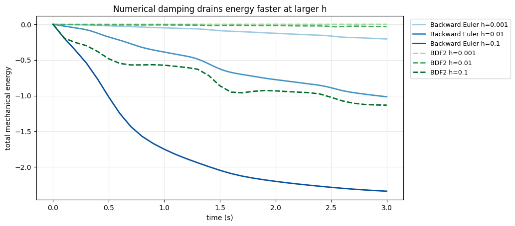
The artificial damping removes mechanical energy. We track elastic + gravitational + kinetic energy (the pins do no work) along the same runs. For Backward Euler, the bigger the timestep, the faster the energy drops; BDF2 (dashed) holds on to far more of it at every timestep.
def mechanical_energy(x, v):
    """Elastic + gravitational + kinetic energy of one state (x, v)."""
    E_elastic = simkit.energies.elastic_energy_x(x.reshape(n, dim), J, mu, lam, vol, MATERIAL)
    E_gravity = -(f_g.T @ x).item()
    E_kinetic = 0.5 * (v.T @ M @ v).item()
    E_total = E_elastic + E_gravity + E_kinetic
    return E_total

fig, ax = plt.subplots(figsize=(9.5, 4.8))
shades = {"Backward Euler": ["#9ecae1", "#4292c6", "#08519c"], "BDF2": ["#a1d99b", "#41ab5d", "#006d2c"]}
for (scheme, h), (ts, xs, vs) in runs.items():
    E = [mechanical_energy(x.reshape(-1, 1), v.reshape(-1, 1)) for x, v in zip(xs, vs)]
    ax.plot(ts, E, color=shades[scheme][DTS.index(h)], lw=2, ls="-" if scheme == "Backward Euler" else "--",
            label=f"{scheme} h={h}")
ax.set_xlabel("time (s)"); ax.set_ylabel("total mechanical energy")
ax.set_title("Numerical damping drains energy faster at larger h")
ax.grid(True, color="0.9"); ax.legend(fontsize=9, loc="upper left", bbox_to_anchor=(1.01, 1.0))
simkit.filesystem.save_figure(fig, os.path.join(RESULTS_DIR, "energy.png"),
                              copy_to=os.path.join(MEDIA_DIR, "007_energy.png"))
plt.show()
Takeaways#
Backward Euler is order 1 and BDF2 order 2, measured on the beam itself.
Forward Euler amplifies the stiffest mode every step and explodes at a timestep the implicit methods handle easily.
Backward Euler damps motion (and drains total energy) more as \(h\) grows; BDF2 stays lively and keeps far more energy.
Every implicit step is one Newton solve of \(V(x) + \tfrac{c}{2h^2}\lVert x - \tilde x\rVert_M^2\); only \(\tilde x\) and \(c\) change.