26 · Sparse Meshless Models: control frames that know the material#
A character is not one material: bones are stiff, flesh is soft, and the two meet at sharp interfaces. A subspace built from geometry alone (radial basis functions, barycentric coordinates, or tutorial 17’s skinning eigenmodes with a uniform stiffness) spreads every control frame’s influence smoothly across those interfaces, so it needs many frames to bend a joint without also bending the bone next to it. Sparse Meshless Models of Complex Deformable Solids (Faure, Gilles, Bousquet, Pai, SIGGRAPH 2011) fixes this with one idea: measure distance in compliance instead of in metres. Two points joined by stiff material are close (they move together), two points joined by soft material are far. Nodes, Voronoi regions and skinning weights all follow from that one metric, and the frames it produces are local: each has compact support and interpolates its node, so a handful of them resolves a heterogeneous body and any one of them can be grabbed as a handle. We compare them against the geometry-only and the material-aware skinning eigenmodes, and against the sparse radial-basis skinning weights of Hyper-Reduced Projective Dynamics (Brandt et al. 2018), which are local like the paper’s frames but geometry-only. Our test body is a tapered tentacle with three stiff segments and two wide soft joints.
Imports, and every tunable parameter of this notebook.
%matplotlib inline
import os
import warnings
import numpy as np
import scipy as sp
import scipy.sparse as sps
import matplotlib.pyplot as plt
from matplotlib.colors import TwoSlopeNorm
import igl
import simkit
import utils

warnings.filterwarnings("ignore", category=sp.linalg.LinAlgWarning)   # stiff pin -> benign ill-conditioning

NOTEBOOK = "026_sparse_meshless_models"                           # this file's name
RESULTS_DIR = utils.notebook_results_path(NOTEBOOK)               # results/026_sparse_meshless_models/
MEDIA_DIR = "media"                                               # tracked copies for the website
# tentacle: a tapered capsule with three stiff segments joined by two soft joints, pinned at its base
LENGTH, R_BASE, R_TIP = 4.0, 0.6, 0.45         # body length and half-thickness at the base / tip (caps added)
SEGMENTS = [(-1.0, 0.9), (1.5, 2.5), (3.1, 5.0)]   # x-ranges of the stiff segments (the 0.6-wide gaps are the joints)
MAX_AREA = 0.004                                # Triangle's maximum triangle area
PIN_X = -0.3                                    # vertices with x <= PIN_X are pinned (inside the base segment)
# material
MATERIAL = "macklin-mueller-neo-hookean"
YM_SOFT, YM_STIFF = 1.0e3, 1.0e6  # Young's modulus of joints / segments (ratio 1000)
PR = 0.4                          # Poisson ratio
RHO = 1.0                         # density
GRAVITY = -9.8                    # vertical gravitational acceleration
K_PIN = 1e9                       # stiffness of the wall pin and of the handle springs
# sparse meshless model
N_NODES = 9                       # control frames; skinning eigenmodes gets the same number of bones
SUPPORT_SCALE = 1.0               # weight support radius / distance to the nearest node (1 = compact tents)
LLOYD_ITERS = 8                   # Lloyd relaxation passes of the node placement
N_WEIGHTS_SHOWN = 3               # weight columns drawn below (the node nearest each stiff segment's centre)
SWEEP_NODES = [3, 6, 9, 12, 18, 24]   # frame counts of the convergence sweep
HRPD_SUPPORT_SCALE = 2.0          # HRPD weight support as a multiple of the sampling's covering distance
# solver and checks
NEWTON_ITERS = 150                # max Newton iterations per solve
NEWTON_TOL = 1e-6                 # stop when the Newton step is shorter than this
PATCH_ANGLE_DEG = 30.0            # rotation of the affine patch test
# handle sweep
N_FRAMES = 36                     # frames of the swing animation
SWING_DEG = 40.0                  # peak angle of the free end's arc
FPS = 12                          # playback rate of the animation
BITRATE = 1800                    # mp4 bitrate
# plot colors
FULL_C, SKIN_C, HRPD_C, SKIN_MAT_C, SM_C = "#d62728", "#7570b3", "#66a61e", "#e6ab02", "#1b9e77"   # full FEM, uniform eigenmodes, HRPD, material eigenmodes, sparse meshless
/home/user/simkit/simkit/__init__.py:262: UserWarning: simkit: some functionality is unavailable because optional dependencies are not installed:
  [viz] (missing: polyscope) -> pip install 'simkit[viz]'
  _emit_missing_warning()
1 · A tentacle with stiff segments and soft joints#
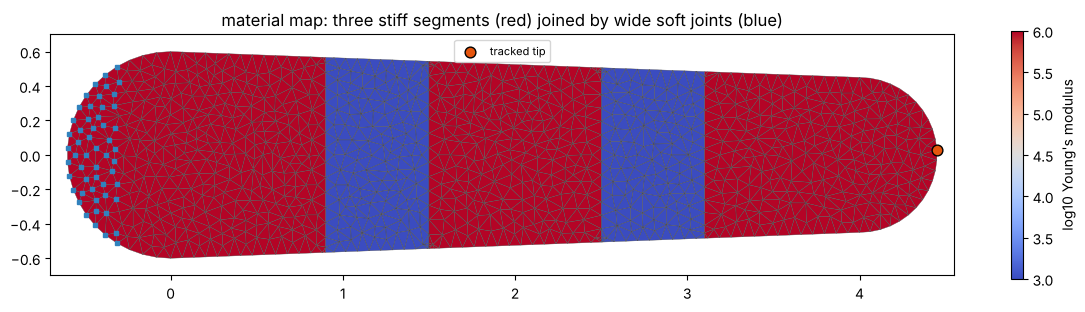
utils.tapered_capsule_mesh meshes a rounded body, \(1.2\) thick at the base and \(0.9\) at the tip, with Triangle, and
tentacle_material assigns each triangle a Young’s modulus by the \(x\) of its centroid: \(10^6\) inside the three
stiff segments (the “bones”) and \(10^3\) in the two \(0.6\)-wide joints between them, a thousand times softer. The
segment boundaries are passed to the mesher as constraint lines so no triangle straddles a material interface.
simkit.ympr_to_lame turns the per-element modulus into the per-element Lamé parameters the elastic energy takes.
The base (blue squares) is pinned; the orange dot is the tip vertex we track.
def tentacle_material(X, T):
    """Per-triangle Young's modulus: YM_STIFF inside SEGMENTS, YM_SOFT in the joints between them."""
    cx = X[T].mean(axis=1)[:, 0]                          # triangle centroid x
    in_segment = np.zeros(len(T), dtype=bool)
    for lo, hi in SEGMENTS:
        in_segment |= (cx >= lo) & (cx <= hi)
    return np.where(in_segment, YM_STIFF, YM_SOFT)

interfaces = [xb for lo, hi in SEGMENTS for xb in (lo, hi)]
X, T = utils.tapered_capsule_mesh(LENGTH, R_BASE, R_TIP, interfaces, max_area=MAX_AREA)
ym = tentacle_material(X, T)
n, dim = X.shape
mu_e, lam_e = simkit.ympr_to_lame(ym, PR)                 # per-element Lame parameters
mu, lam = mu_e.reshape(-1, 1), lam_e.reshape(-1, 1)
pin_idx = np.where(X[:, 0] <= PIN_X)[0]
handle_idx = np.where(X[:, 0] >= LENGTH)[0]               # the tip cap
tip = int(np.argmax(X[:, 0]))
print(f"tentacle: {n} vertices, {len(T)} triangles, {X.size} DOFs; "
      f"{(ym == YM_STIFF).sum()} stiff triangles, {(ym == YM_SOFT).sum()} soft triangles")

fig, ax = plt.subplots(figsize=(12, 3.4))
utils.plot_scalar_field(ax, X, T, np.log10(ym), cmap="coolwarm", edges=True, label="log10 Young's modulus",
                        title="material map: three stiff segments (red) joined by wide soft joints (blue)")
ax.plot(*X[pin_idx].T, "s", color=utils.PIN_C, ms=3, zorder=6)
ax.scatter(*X[tip], s=60, color=utils.HANDLE_C, edgecolors="k", zorder=6, label="tracked tip")
ax.legend(loc="upper center", fontsize=8)
fig.tight_layout()
simkit.filesystem.save_figure(fig, os.path.join(RESULTS_DIR, "material.png"),
                              copy_to=os.path.join(MEDIA_DIR, "026_material.png"))
plt.show()
tentacle: 1093 vertices, 2010 triangles, 2186 DOFs; 1514 stiff triangles, 496 soft triangles
2 · The compliance distance#
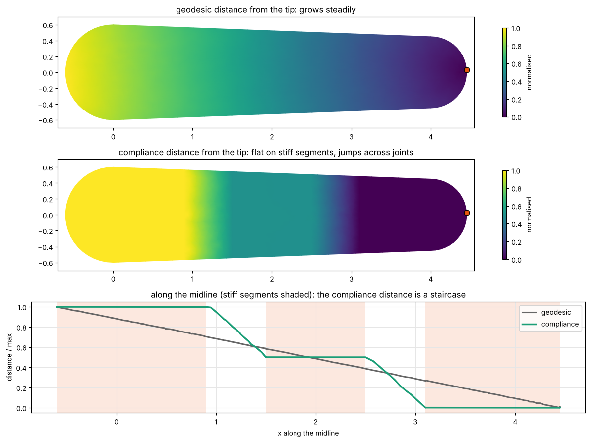
simkit.compliance_graph weights every mesh edge by its length times the compliance \(1/E\) of the triangles it borders,
and simkit.compliance_distances runs Dijkstra on that graph. Measured from the tip (orange), the ordinary geodesic
distance grows steadily along the body, while the compliance distance barely moves inside a stiff segment and jumps
across each joint: in this metric a segment is nearly a single point and the tentacle is a chain of three points joined
by two long soft springs. The lower plot follows both distances along the midline, each normalised to its maximum.
G_compliance = simkit.compliance_graph(X, T, ym)                   # edge weights: length / E
G_geodesic = simkit.compliance_graph(X, T, np.ones(len(T)))         # uniform material -> plain edge lengths
d_compliance = simkit.compliance_distances(G_compliance, tip)[0]
d_geodesic = simkit.compliance_distances(G_geodesic, tip)[0]

mid_row = np.where(np.abs(X[:, 1]) < 0.06)[0]                     # vertices near the midline y = 0
mid_row = mid_row[np.argsort(X[mid_row, 0])]
fig, axes = plt.subplots(3, 1, figsize=(12, 9.0), gridspec_kw={"height_ratios": [1, 1, 1.0]})
utils.plot_scalar_field(axes[0], X, T, d_geodesic / d_geodesic.max(), edges=False, label="normalised",
                        title="geodesic distance from the tip: grows steadily")
utils.plot_scalar_field(axes[1], X, T, d_compliance / d_compliance.max(), edges=False, label="normalised",
                        title="compliance distance from the tip: flat on stiff segments, jumps across joints")
for ax in axes[:2]:
    ax.scatter(*X[tip], s=60, color=utils.HANDLE_C, edgecolors="k", zorder=6)
axes[2].plot(X[mid_row, 0], d_geodesic[mid_row] / d_geodesic.max(), color="0.4", lw=2.2, label="geodesic")
axes[2].plot(X[mid_row, 0], d_compliance[mid_row] / d_compliance.max(), color=SM_C, lw=2.5, label="compliance")
for lo, hi in SEGMENTS:
    axes[2].axvspan(max(lo, X[:, 0].min()), min(hi, X[:, 0].max()), color="#f4a582", alpha=0.25, lw=0)
axes[2].set_xlabel("x along the midline"); axes[2].set_ylabel("distance / max")
axes[2].set_title("along the midline (stiff segments shaded): the compliance distance is a staircase")
axes[2].grid(True, color="0.9"); axes[2].legend(loc="upper right")
fig.tight_layout()
simkit.filesystem.save_figure(fig, os.path.join(RESULTS_DIR, "distances.png"),
                              copy_to=os.path.join(MEDIA_DIR, "026_distances.png"))
plt.show()
3 · Placing the control nodes where the compliance is#
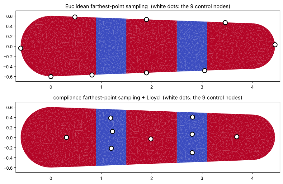
simkit.compliance_node_sampling runs farthest-point sampling in the compliance metric and then Lloyd relaxation (each
node moves to the centre of its region), the compliance analogue of simkit.farthest_point_sampling. Because a stiff
segment is tiny in this metric and a joint is long, the same nine nodes land differently: Euclidean sampling spreads
them evenly over the body, compliance sampling spends most of them on the joints, where the deformation will actually
happen, and gives each stiff segment no more than it needs.
nodes_euclid = simkit.farthest_point_sampling(X, N_NODES)
nodes = simkit.compliance_node_sampling(X, G_compliance, N_NODES, lloyd_iters=LLOYD_ITERS)

def in_joint(idx):
    """True for the nodes whose x lies in a joint (outside every stiff segment)."""
    x = X[idx, 0]
    inside = np.zeros(len(idx), dtype=bool)
    for lo, hi in SEGMENTS:
        inside |= (x >= lo) & (x <= hi)
    return ~inside

def one_per_segment(idx):
    """For each stiff segment, the index (into idx) of the node nearest its centre, if it has one."""
    chosen = []
    for lo, hi in SEGMENTS:
        inside = np.where((X[idx, 0] >= lo) & (X[idx, 0] <= hi))[0]
        if inside.size:
            chosen.append(int(inside[np.argmin(np.abs(X[idx[inside], 0] - 0.5 * (max(lo, X[:, 0].min()) + min(hi, X[:, 0].max()))))]))
    return chosen[:N_WEIGHTS_SHOWN]

print(f"Euclidean sampling : {in_joint(nodes_euclid).sum()} of {N_NODES} nodes in the joints")
print(f"compliance sampling: {in_joint(nodes).sum()} of {N_NODES} nodes in the joints")

fig, axes = plt.subplots(2, 1, figsize=(12, 6.0))
for ax, idx, name in zip(axes, [nodes_euclid, nodes], ["Euclidean farthest-point sampling",
                                                       "compliance farthest-point sampling + Lloyd"]):
    utils.plot_scalar_field(ax, X, T, np.log10(ym), cmap="coolwarm", edges=False, colorbar=False,
                            title=f"{name}  (white dots: the {N_NODES} control nodes)")
    ax.scatter(*X[idx].T, s=110, color="k", marker="o", zorder=6)
    ax.scatter(*X[idx].T, s=50, color="w", marker="o", zorder=7)
fig.tight_layout()
simkit.filesystem.save_figure(fig, os.path.join(RESULTS_DIR, "nodes.png"),
                              copy_to=os.path.join(MEDIA_DIR, "026_nodes.png"))
plt.show()
Euclidean sampling : 1 of 9 nodes in the joints
compliance sampling: 6 of 9 nodes in the joints
4 · Voronoi regions and material-aware skinning weights#
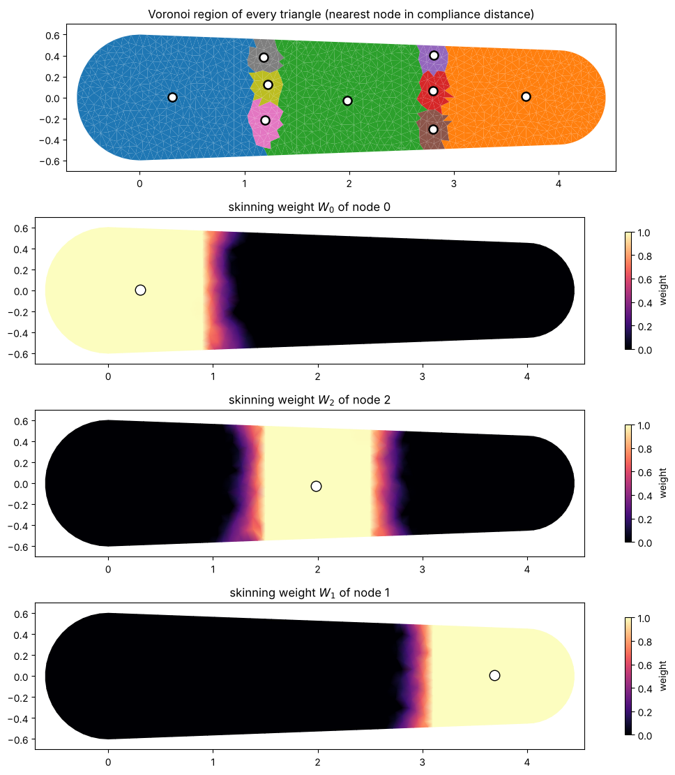
With the node-to-vertex compliance distances in hand, simkit.voronoi_labels assigns every triangle to its nearest node
and simkit.voronoi_shape_functions builds the skinning weights: each node gets a clamped-linear tent in the compliance
metric (\(1\) at the node, \(\tfrac12\) at the Voronoi frontier, \(0\) at the nearest other node), normalised to a partition of
unity. Crossing a joint is expensive, so a segment node’s weight is constant across its segment and fades linearly
through the joint, and a joint node’s weight never leaks into the stiff segments. The printout checks the three
properties a skinning basis needs; the figure shows the Voronoi regions and the weight of one node per stiff segment.
D_nodes = simkit.compliance_distances(G_compliance, nodes)                 # (k, n)
vertex_labels, face_labels = simkit.voronoi_labels(D_nodes, T)
W = simkit.voronoi_shape_functions(D_nodes, nodes, support_scale=SUPPORT_SCALE)  # sparse (n, k)
k = len(nodes)
bone_nodes = one_per_segment(nodes)
print(f"W: {W.shape}, {W.nnz} non-zeros ({W.nnz / np.prod(W.shape) * 100:.0f}% dense)")
print(f"  partition of unity : max |row sum - 1| = {np.abs(W.sum(axis=1).A.ravel() - 1).max():.1e}")
print(f"  non-negative       : min W = {W.min():.1e}")
print(f"  interpolating      : max |W[nodes] - I| = {np.abs(W[nodes].toarray() - np.eye(k)).max():.1e}")

fig, axes = plt.subplots(1 + len(bone_nodes), 1, figsize=(12, 2.8 * (1 + len(bone_nodes))))
utils.plot_scalar_field(axes[0], X, T, face_labels, cmap="tab10", vmin=-0.5, vmax=9.5, edges=False, colorbar=False,
                        title="Voronoi region of every triangle (nearest node in compliance distance)")
axes[0].scatter(*X[nodes].T, s=90, color="k", zorder=6); axes[0].scatter(*X[nodes].T, s=36, color="w", zorder=7)
for ax, j in zip(axes[1:], bone_nodes):
    utils.plot_scalar_field(ax, X, T, W[:, j].toarray().ravel(), cmap="magma", vmin=0, vmax=1, edges=False,
                            label="weight", title=f"skinning weight $W_{{{j}}}$ of node {j}")
    ax.scatter(*X[nodes[j]], s=110, color="w", edgecolors="k", zorder=6)
fig.tight_layout()
simkit.filesystem.save_figure(fig, os.path.join(RESULTS_DIR, "weights.png"),
                              copy_to=os.path.join(MEDIA_DIR, "026_weights.png"))
plt.show()
W: (1093, 9), 2699 non-zeros (27% dense)
  partition of unity : max |row sum - 1| = 2.2e-16
  non-negative       : min W = 0.0e+00
  interpolating      : max |W[nodes] - I| = 0.0e+00
5 · A sparse skinning subspace#
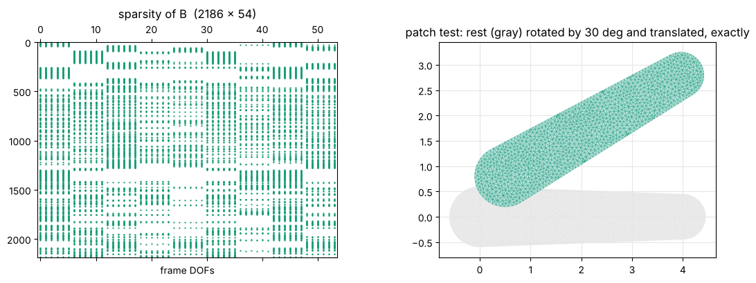
Each node carries a \(2\times3\) affine frame, so the subspace is \(x = B\,z\) with \(r = 6k\) coordinates. Tutorial 17
built this \(B\) dense with simkit.lbs_jacobian; the same call with sparse=True assembles only the non-zeros of \(W\) and
returns a csr_matrix with the identical layout, which is what keeps a model with hundreds of local frames cheap. The
printout checks that the two agree. Then the patch test: because the weights sum to one, giving every frame the same
affine map \([A \mid t]\) reproduces that map on the whole body. In lbs_jacobian’s layout each frame’s six DOFs are the
columns of \([A \mid t]\) in order, so affine_coordinates is one np.tile. The rest state is the identity map, so no
projection is needed to start a simulation in this subspace.
B_sm = simkit.lbs_jacobian(X, W, sparse=True)                   # (n*dim, 6k), sparse
B_dense = simkit.lbs_jacobian(X, W.toarray())                   # the same, dense
print(f"B: {B_sm.shape}, {B_sm.nnz} non-zeros ({B_sm.nnz / np.prod(B_sm.shape) * 100:.0f}% dense); "
      f"max |sparse - dense| = {np.abs(B_sm.toarray() - B_dense).max():.1e}")

def affine_coordinates(k, A, t):
    """Subspace coordinates z that give all k frames the same affine map x -> A x + t."""
    return np.tile(np.c_[A, t].T.ravel(), k).reshape(-1, 1)

th = np.deg2rad(PATCH_ANGLE_DEG)
R = np.array([[np.cos(th), -np.sin(th)], [np.sin(th), np.cos(th)]])
t_patch = np.array([0.5, 0.8])
z_patch = affine_coordinates(k, R, t_patch)                     # every frame = the same map x -> R x + t
x_patch = (B_sm @ z_patch).reshape(n, dim)
z_rest = affine_coordinates(k, np.eye(dim), np.zeros(dim))
print(f"patch test: max |B z - (R X + t)| = {np.abs(x_patch - (X @ R.T + t_patch)).max():.1e};  "
      f"rest: max |B z_rest - X| = {np.abs((B_sm @ z_rest).reshape(n, dim) - X).max():.1e}")

fig, (axL, axR) = plt.subplots(1, 2, figsize=(12, 4.2), gridspec_kw={"width_ratios": [1, 1.6]})
axL.spy(B_sm, markersize=0.6, color=SM_C, aspect="auto")
axL.set_title(f"sparsity of B  ({B_sm.shape[0]} x {B_sm.shape[1]})"); axL.set_xlabel("frame DOFs")
lims = utils.auto_limits([X, x_patch], pad=0.2)
utils.PolyMeshArtist(axR, X, T, facecolor="0.9", edgecolor="none", zorder=1)
utils.plot_mesh(axR, x_patch, T, lims=lims, lw=0.3, facecolor="#b2dfdb", edgecolor=SM_C,
                title=f"patch test: rest (gray) rotated by {PATCH_ANGLE_DEG:.0f} deg and translated, exactly")
fig.tight_layout()
simkit.filesystem.save_figure(fig, os.path.join(RESULTS_DIR, "subspace.png"),
                              copy_to=os.path.join(MEDIA_DIR, "026_subspace.png"))
plt.show()
B: (2186, 54), 16194 non-zeros (14% dense); max |sparse - dense| = 0.0e+00
patch test: max |B z - (R X + t)| = 1.8e-15;  rest: max |B z_rest - X| = 8.9e-16
6 · A geometry-only sparse basis: Hyper-Reduced Projective Dynamics#
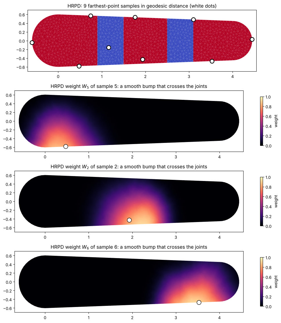
Hyper-Reduced Projective Dynamics (Brandt, Eisemann, Hildebrandt, SIGGRAPH 2018) also builds a sparse skinning subspace
with no training data and no eigenproblem, but from geometry only: sample vertices by farthest-point sampling in the
geodesic distance, give each sample a compactly supported radial basis function of that distance (a Wendland kernel with
support radius HRPD_SUPPORT_SCALE times the sampling’s covering distance), normalise to a partition of unity, and attach
an affine frame per sample. simkit.hyper_reduced_projective_dynamics_basis does exactly that; its weights are smooth
bumps that ignore the material, so they straddle the joints instead of stopping at them. The figure shows the samples
and one weight per stiff segment, next to the sparse meshless weights of the same nodes for comparison.
W_hrpd, B_hrpd, samples_hrpd, D_hrpd = simkit.hyper_reduced_projective_dynamics_basis(
    X, T, N_NODES, support_scale=HRPD_SUPPORT_SCALE, return_distances=True)
print(f"HRPD: {len(samples_hrpd)} samples, W {W_hrpd.shape} ({W_hrpd.nnz / np.prod(W_hrpd.shape) * 100:.0f}% dense), "
      f"B {B_hrpd.shape} ({B_hrpd.nnz / np.prod(B_hrpd.shape) * 100:.0f}% dense)")
print(f"  partition of unity : max |row sum - 1| = {np.abs(W_hrpd.sum(axis=1).A.ravel() - 1).max():.1e}")
print(f"  non-negative       : min W = {W_hrpd.min():.1e}")
print(f"  samples in joints  : {in_joint(samples_hrpd).sum()} of {N_NODES}")

hrpd_shown = one_per_segment(samples_hrpd)
fig, axes = plt.subplots(1 + len(hrpd_shown), 1, figsize=(12, 2.8 * (1 + len(hrpd_shown))))
utils.plot_scalar_field(axes[0], X, T, np.log10(ym), cmap="coolwarm", edges=False, colorbar=False,
                        title=f"HRPD: {N_NODES} farthest-point samples in geodesic distance (white dots)")
axes[0].scatter(*X[samples_hrpd].T, s=110, color="k", zorder=6); axes[0].scatter(*X[samples_hrpd].T, s=50, color="w", zorder=7)
for ax, j in zip(axes[1:], hrpd_shown):
    utils.plot_scalar_field(ax, X, T, W_hrpd[:, j].toarray().ravel(), cmap="magma", vmin=0, vmax=1, edges=False,
                            label="weight", title=f"HRPD weight $W_{{{j}}}$ of sample {j}: a smooth bump that crosses the joints")
    ax.scatter(*X[samples_hrpd[j]], s=110, color="w", edgecolors="k", zorder=6)
fig.tight_layout()
simkit.filesystem.save_figure(fig, os.path.join(RESULTS_DIR, "hrpd_weights.png"),
                              copy_to=os.path.join(MEDIA_DIR, "026_hrpd_weights.png"))
plt.show()
HRPD: 9 samples, W (1093, 9) (51% dense), B (2186, 54) (26% dense)
  partition of unity : max |row sum - 1| = 7.0e-10
  non-negative       : min W = 0.0e+00
  samples in joints  : 1 of 9
7 · Statics in five spaces#
tentacle_operators builds the constant operators once: the deformation Jacobian, triangle areas, the per-element Lamé
parameters, the lumped mass matrix (for mass-norm errors), the gravity force and the soft pin at the base.
subspace_statics_system is the elastostatic problem of tutorial 4 written in subspace coordinates, \(x = Bz + q\),
with full integration and a Galerkin projection of the gradient and Hessian; with \(B = I\) it is the full FEM problem.
Each term is its own line and the total sums them.
def tentacle_operators(X, T, mu, lam):
    """Constant operators of the pinned heterogeneous tentacle, built once from simkit."""
    n, dim = X.shape
    Q_pin, b_pin = simkit.dirichlet_penalty(pin_idx, X[pin_idx], n, K_PIN)
    M_vertex = simkit.massmatrix(X, T, rho=RHO)
    ops = {
        "n": n, "dim": dim,
        "J": simkit.deformation_jacobian(X, T),
        "vol": simkit.volume(X, T),
        "mu": mu, "lam": lam,
        "M": sp.sparse.kron(M_vertex, sp.sparse.eye(dim)).tocsc(),
        "f_g": simkit.gravity_force(X, T, a=GRAVITY, rho=RHO).reshape(-1, 1),
        "Q_pin": Q_pin, "b_pin": b_pin,
    }
    return ops

def subspace_statics_system(ops, B, q, handle_targets=None):
    """Elastostatics (gravity + base pin + optional handle) in subspace coordinates z, where x = B z + q."""
    n, dim = ops["n"], ops["dim"]
    J, vol, mu, lam = ops["J"], ops["vol"], ops["mu"], ops["lam"]
    f_g, Q_pin, b_pin = ops["f_g"], ops["Q_pin"], ops["b_pin"]
    if handle_targets is None:
        Q_h, b_h = sp.sparse.csc_matrix((n * dim, n * dim)), np.zeros((n * dim, 1))
    else:
        Q_h, b_h = simkit.dirichlet_penalty(handle_idx, handle_targets, n, K_PIN)

    def energy_func(z):
        x = B @ z + q
        E_elastic = simkit.energies.elastic_energy_x(x.reshape(n, dim), J, mu, lam, vol, MATERIAL)
        E_gravity = -(f_g.T @ x).item()
        E_pin = simkit.energies.quadratic_energy(x, Q_pin, b_pin)
        E_handle = simkit.energies.quadratic_energy(x, Q_h, b_h)
        E_total = E_elastic + E_gravity + E_pin + E_handle
        return E_total

    def gradient_func(z):
        x = B @ z + q
        g_elastic = simkit.energies.elastic_gradient_x(x.reshape(n, dim), J, mu, lam, vol, MATERIAL)
        g_gravity = -f_g
        g_pin = simkit.energies.quadratic_gradient(x, Q_pin, b_pin)
        g_handle = simkit.energies.quadratic_gradient(x, Q_h, b_h)
        g_total = g_elastic + g_gravity + g_pin + g_handle
        g_z = B.T @ g_total                                   # Galerkin projection
        return g_z

    def hessian_func(z):
        x = B @ z + q
        H_elastic = simkit.energies.elastic_hessian_x(x.reshape(n, dim), J, mu, lam, vol, MATERIAL, psd=True)
        H_pin = simkit.energies.quadratic_hessian(Q_pin)
        H_handle = simkit.energies.quadratic_hessian(Q_h)
        H_total = H_elastic + H_pin + H_handle
        H_z = B.T @ (H_total @ B)                             # Galerkin projection
        return H_z

    return energy_func, gradient_func, hessian_func

ops = tentacle_operators(X, T, mu, lam)
Five spaces, all with the same nine bones so the four subspaces have exactly \(54\) DOFs:
full FEM (\(B = I\)), the reference;
uniform skinning eigenmodes (
simkit.skinning_eigenmodes(X, T, k), tutorial 17): Laplacian eigenvectors of the geometry, which know nothing about the material;HRPD (
simkit.hyper_reduced_projective_dynamics_basis): the sparse radial-basis skinning weights above, also geometry-only but local;material skinning eigenmodes (
simkit.skinning_eigenmodes(X, T, k, mu=mu)): the same eigenproblem on the Laplacian weighted by the per-element stiffness \(\mu\), so the modes are nearly constant on the stiff segments and vary in the joints. They are smooth and global: every bone’s weight is non-zero everywhere, and \(B\) is dense;sparse meshless frames, started from \(z_{\text{rest}}\); the eigenmode and HRPD spaces start from the mass-norm projection of the rest shape.
solve_statics runs Newton with line search from a given start, and we let the tentacle sag under gravity in each space.
The error is the relative mass-norm distance to the full solution; the printout also lists how dense each \(B\) is.
x_rest = X.reshape(-1, 1)
_, _, B_skin = simkit.skinning_eigenmodes(X, T, N_NODES)             # geometry only: uniform stiffness
_, _, B_skin_mat = simkit.skinning_eigenmodes(X, T, N_NODES, mu=mu)  # material-aware: Laplacian weighted by mu
spaces = {
    f"full FEM  ({X.size} DOFs)": (sp.sparse.identity(X.size, format="csc"), np.zeros((X.size, 1)), x_rest.copy()),
    f"uniform skinning eigenmodes  ({B_skin.shape[1]} DOFs)": (B_skin, np.zeros((X.size, 1)),
                                                                simkit.project_into_subspace(x_rest, B_skin, M=ops["M"])),
    f"HRPD  ({B_hrpd.shape[1]} DOFs)": (B_hrpd, np.zeros((X.size, 1)),
                                        simkit.project_into_subspace(x_rest, B_hrpd, M=ops["M"])),
    f"material skinning eigenmodes  ({B_skin_mat.shape[1]} DOFs)": (B_skin_mat, np.zeros((X.size, 1)),
                                                                     simkit.project_into_subspace(x_rest, B_skin_mat, M=ops["M"])),
    f"sparse meshless  ({B_sm.shape[1]} DOFs)": (B_sm, np.zeros((X.size, 1)), z_rest.copy()),
}
space_colors = dict(zip(spaces, [FULL_C, SKIN_C, HRPD_C, SKIN_MAT_C, SM_C]))
for name, (B, _, _) in list(spaces.items())[1:]:
    nnz = B.nnz if sps.issparse(B) else np.count_nonzero(B)
    print(f"{name:44s}: B is {nnz / np.prod(B.shape) * 100:3.0f}% dense")

def solve_statics(B, q, z0, handle_targets=None):
    """Newton solve of the static tentacle in the subspace x = B z + q, from z0. Returns (x, z, iterations)."""
    system = subspace_statics_system(ops, B, q, handle_targets)
    z, info = simkit.solvers.newton_solver(z0, *system, tolerance=NEWTON_TOL, max_iter=NEWTON_ITERS,
                                           do_line_search=True, return_info=True)
    x = (B @ z + q).reshape(n, dim)
    return x, z, info["iters"] + 1

def mass_norm_error(x, x_ref):
    """Relative mass-norm distance between two stacked positions."""
    d = (x - x_ref).reshape(-1, 1)
    M = ops["M"]
    return np.sqrt((d.T @ M @ d).item() / (x_ref.reshape(-1, 1).T @ M @ x_ref.reshape(-1, 1)).item())

sag = {}
for name, (B, q, z0) in spaces.items():
    sag[name], _, iters = solve_statics(B, q, z0)
    print(f"{name:44s}: tip height {sag[name][tip, 1]:+.3f}, {iters} Newton iterations")
x_full = sag[next(iter(spaces))]
for name in list(spaces)[1:]:
    print(f"{name:44s}: relative mass-norm error vs full = {mass_norm_error(sag[name], x_full):.3f}")
uniform skinning eigenmodes  (54 DOFs)      : B is  50% dense
HRPD  (54 DOFs)                             : B is  26% dense
material skinning eigenmodes  (54 DOFs)     : B is  50% dense
sparse meshless  (54 DOFs)                  : B is  14% dense
full FEM  (2186 DOFs)                       : tip height -0.772, 31 Newton iterations
uniform skinning eigenmodes  (54 DOFs)      : tip height +0.026, 3 Newton iterations
HRPD  (54 DOFs)                             : tip height +0.025, 3 Newton iterations
material skinning eigenmodes (54 DOFs) : tip height -0.741, 28 Newton iterations
sparse meshless  (54 DOFs)                  : tip height -0.477, 22 Newton iterations
uniform skinning eigenmodes  (54 DOFs)      : relative mass-norm error vs full = 0.149
HRPD  (54 DOFs)                             : relative mass-norm error vs full = 0.149
material skinning eigenmodes  (54 DOFs)     : relative mass-norm error vs full = 0.006
sparse meshless  (54 DOFs)                  : relative mass-norm error vs full = 0.054
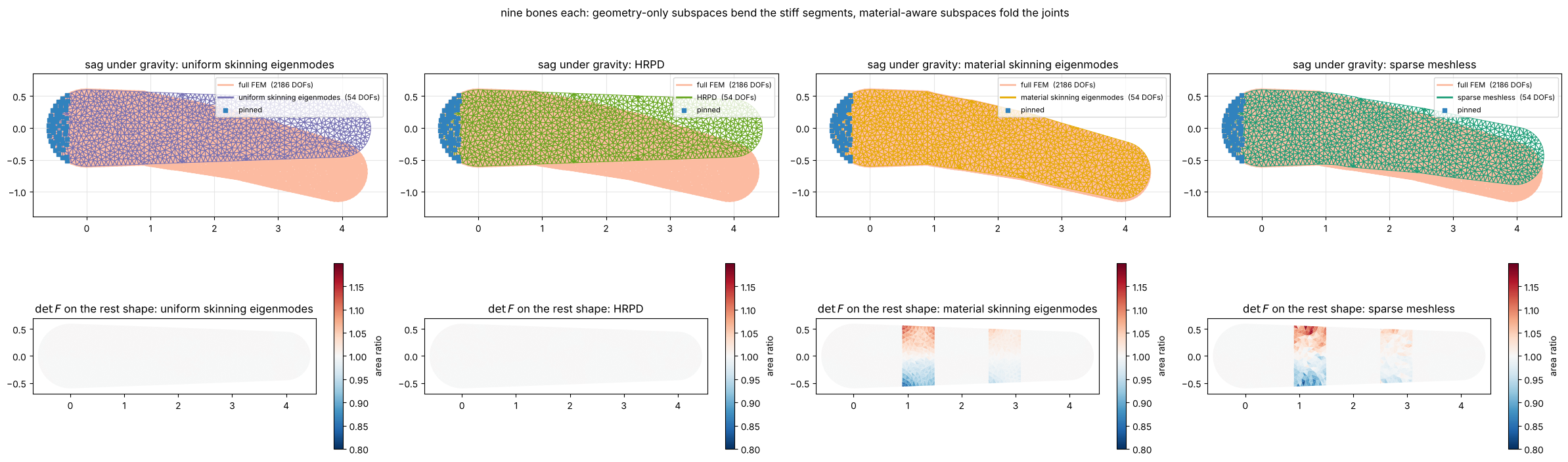
The sag, each subspace (thin, coloured) over the full solution (thick, light red), and below it the strain of every triangle (area ratio \(\det F\) on the rest shape). The four subspaces have the same \(54\) DOFs and tell four stories:
Uniform skinning eigenmodes bend the body smoothly everywhere, stiff segments included; bending a segment costs a thousand times more than bending a joint, so the subspace barely moves and strains nothing.
HRPD is local but still geometry-only: every bump straddles a joint, so folding a joint also bends the segments on either side, and the subspace stays almost as rigid as the uniform eigenmodes.
Material skinning eigenmodes put all their variation in the joints and land almost on the full solution. With the material in the Laplacian, a smooth global basis is an excellent subspace for this body.
Sparse meshless frames keep the segments straight and fold both joints, recovering well over half of the sag. What is missing is the shape of the fold: inside a joint the model can only blend two affine frames linearly in compliance distance, while the full solve bends with a smooth profile.
The sparse frames buy something the eigenmodes do not offer: each one is local (its weight is zero outside its own neighbourhood, so \(B\) is a sparse matrix) and interpolates its node, so a frame can be grabbed directly as a handle. HRPD shares the sparsity; what it lacks is the material in its metric.
lims = utils.auto_limits(list(sag.values()), pad=0.25)
names = list(spaces)
fig, axes = plt.subplots(2, 4, figsize=(24, 7.4))
for ax, name in zip(axes[0], names[1:]):
    utils.plot_mesh_overlay(ax, {names[0]: x_full, name: sag[name]}, T,
                            colors={names[0]: "#fcbba1", name: space_colors[name]}, lws={names[0]: 3.0, name: 0.7},
                            pin_pts=X[pin_idx], lims=lims, title=f"sag under gravity: {name.split('  ')[0]}")
    ax.legend(loc="upper right", fontsize=8)
area_ratio = {name: np.linalg.det((ops["J"] @ x.reshape(-1, 1)).reshape(-1, dim, dim)) for name, x in sag.items()}
norm = TwoSlopeNorm(vmin=0.8, vcenter=1.0, vmax=1.2)
for ax, name in zip(axes[1], names[1:]):
    utils.plot_scalar_field(ax, X, T, area_ratio[name], cmap="RdBu_r", norm=norm, edges=False, label="area ratio",
                            title=f"$\\det F$ on the rest shape: {name.split('  ')[0]}")
fig.suptitle("nine bones each: geometry-only subspaces bend the stiff segments, material-aware subspaces fold the joints")
fig.tight_layout()
simkit.filesystem.save_figure(fig, os.path.join(RESULTS_DIR, "sag.png"),
                              copy_to=os.path.join(MEDIA_DIR, "026_sag.png"))
plt.show()
8 · Does adding frames fix it?#
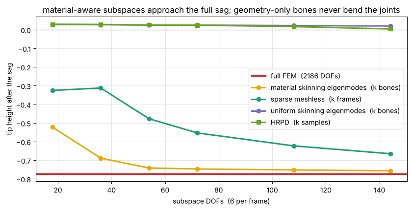
sag_in_subspace repeats the gravity solve for the four subspaces at each frame count of the sweep (same number of
bones, so the same DOFs) and we plot the tip height against the full solve. The material skinning eigenmodes are within a
few percent from six bones on. The sparse meshless model approaches the full solution more slowly as frames are added,
mostly inside the joints where the compliance metric puts them; the curve is not monotone at small counts because
farthest-point sampling decides where each extra frame lands. The two geometry-only bases, uniform eigenmodes and
HRPD, stay rigid at every size: a weight that ignores the material has to bend a stiff segment to bend a joint.
def sag_in_subspace(k):
    """Tip height of the gravity sag with k sparse meshless frames, k uniform / material eigenmode bones and k HRPD samples."""
    nodes_k = simkit.compliance_node_sampling(X, G_compliance, k, lloyd_iters=LLOYD_ITERS)
    W_k = simkit.voronoi_shape_functions(simkit.compliance_distances(G_compliance, nodes_k), nodes_k,
                                         support_scale=SUPPORT_SCALE)
    B_k = simkit.lbs_jacobian(X, W_k, sparse=True)
    x_sm, _, _ = solve_statics(B_k, np.zeros((X.size, 1)), affine_coordinates(k, np.eye(dim), np.zeros(dim)))
    _, _, B_sk = simkit.skinning_eigenmodes(X, T, k)
    x_sk, _, _ = solve_statics(B_sk, np.zeros((X.size, 1)), simkit.project_into_subspace(x_rest, B_sk, M=ops["M"]))
    _, _, B_skm = simkit.skinning_eigenmodes(X, T, k, mu=mu)
    x_skm, _, _ = solve_statics(B_skm, np.zeros((X.size, 1)), simkit.project_into_subspace(x_rest, B_skm, M=ops["M"]))
    _, B_hr, _ = simkit.hyper_reduced_projective_dynamics_basis(X, T, k, support_scale=HRPD_SUPPORT_SCALE)
    x_hr, _, _ = solve_statics(B_hr, np.zeros((X.size, 1)), simkit.project_into_subspace(x_rest, B_hr, M=ops["M"]))
    return x_sm[tip, 1], x_sk[tip, 1], x_skm[tip, 1], x_hr[tip, 1]

sweep = np.array([sag_in_subspace(k) for k in SWEEP_NODES])
dofs = 6 * np.array(SWEEP_NODES)
for k, (t_sm, t_sk, t_skm, t_hr) in zip(SWEEP_NODES, sweep):
    print(f"k={k:2d} ({6 * k:3d} DOFs): sparse meshless {t_sm / x_full[tip, 1] * 100:3.0f}% of the full sag, "
          f"uniform skinning {t_sk / x_full[tip, 1] * 100:3.0f}%, HRPD {t_hr / x_full[tip, 1] * 100:3.0f}%, "
          f"material skinning {t_skm / x_full[tip, 1] * 100:3.0f}%")

fig, ax = plt.subplots(figsize=(8.5, 4.4))
ax.axhline(x_full[tip, 1], color=FULL_C, lw=2.5, label=f"full FEM  ({X.size} DOFs)")
ax.plot(dofs, sweep[:, 2], "-o", color=SKIN_MAT_C, lw=2.2, ms=6, label="material skinning eigenmodes  (k bones)")
ax.plot(dofs, sweep[:, 0], "-o", color=SM_C, lw=2.2, ms=6, label="sparse meshless  (k frames)")
ax.plot(dofs, sweep[:, 1], "-o", color=SKIN_C, lw=2.2, ms=6, label="uniform skinning eigenmodes  (k bones)")
ax.plot(dofs, sweep[:, 3], "-s", color=HRPD_C, lw=2.2, ms=6, label="HRPD  (k samples)")
ax.axhline(0.0, color="0.7", lw=1, ls="--")
ax.set_xlabel("subspace DOFs  (6 per frame)"); ax.set_ylabel("tip height after the sag")
ax.set_title("material-aware subspaces approach the full sag; geometry-only bones never bend the joints")
ax.grid(True, color="0.9"); ax.legend(loc="center right")
fig.tight_layout()
simkit.filesystem.save_figure(fig, os.path.join(RESULTS_DIR, "convergence.png"),
                              copy_to=os.path.join(MEDIA_DIR, "026_convergence.png"))
plt.show()
k= 3 ( 18 DOFs): sparse meshless  42% of the full sag, uniform skinning  -4%, HRPD  -4%, material skinning  68%
k= 6 ( 36 DOFs): sparse meshless  40% of the full sag, uniform skinning  -4%, HRPD  -4%, material skinning  89%
k= 9 ( 54 DOFs): sparse meshless  62% of the full sag, uniform skinning  -3%, HRPD  -3%, material skinning  96%
k=12 ( 72 DOFs): sparse meshless  72% of the full sag, uniform skinning  -3%, HRPD  -3%, material skinning  97%
k=18 (108 DOFs): sparse meshless  81% of the full sag, uniform skinning  -3%, HRPD  -2%, material skinning  97%
k=24 (144 DOFs): sparse meshless  86% of the full sag, uniform skinning  -3%, HRPD  -1%, material skinning  98%
9 · Swinging the free end#
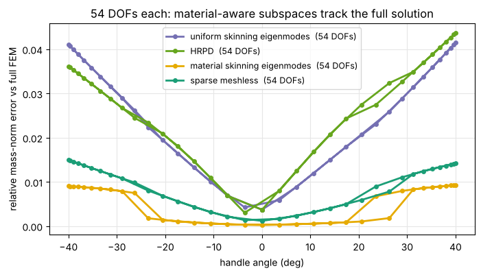
A stiff handle drags the tip cap of the tentacle (rotated about the base) through an arc of \(\pm40^\circ\), re-solving the statics in each space at every frame, warm-started from the previous one. The animation plays the five spaces side by side with the full solution ghosted in gray under each subspace, and the plot tracks each subspace’s error over the sweep. The handle fixes where the tip goes, so every subspace is close to the full solution there; the difference is in between, where the two material-aware subspaces fold the joints and the geometry-only bases bend the segments.
angles = np.deg2rad(SWING_DEG) * np.sin(np.linspace(0, 2 * np.pi, N_FRAMES))
pivot = X[pin_idx].mean(axis=0)
states = {name: [] for name in spaces}
errors = {name: [] for name in names[1:]}
z_curr = {name: z0.copy() for name, (_, _, z0) in spaces.items()}
for th in angles:
    R = np.array([[np.cos(th), -np.sin(th)], [np.sin(th), np.cos(th)]])
    targets = (X[handle_idx] - pivot) @ R.T + pivot             # tip cap swung about the pinned base
    for name, (B, q, _) in spaces.items():
        x, z_curr[name], _ = solve_statics(B, q, z_curr[name], targets)
        states[name].append(x)
    for name in names[1:]:
        errors[name].append(mass_norm_error(states[name][-1], states[names[0]][-1]))
for name in names[1:]:
    print(f"{name:44s}: mean error over the sweep {np.mean(errors[name]):.3f}, max {np.max(errors[name]):.3f}")

lims = utils.auto_limits(sum(states.values(), []), pad=0.2)
panels = [{"states": states[names[0]], "T": T, "title": names[0], "color": "#fcbba1"}]
for name in names[1:]:
    panels.append({"states": states[name], "T": T, "title": name, "color": space_colors[name],
                   "ghost": states[names[0]]})
fig, anim = utils.animate_colored_mesh_panels(panels, lims=lims, fps=FPS, figsize=(24, 5.0),
                                              suptitle="the free end swung through an arc, solved in five spaces")
video = simkit.filesystem.save_animation(anim, os.path.join(RESULTS_DIR, "swing.mp4"), fps=FPS, bitrate=BITRATE,
                                         copy_to=os.path.join(MEDIA_DIR, "026_swing.mp4"))
plt.close(fig)
utils.embed_video(video)
uniform skinning eigenmodes  (54 DOFs)      : mean error over the sweep 0.025, max 0.041
HRPD  (54 DOFs)                             : mean error over the sweep 0.026, max 0.044
material skinning eigenmodes  (54 DOFs)     : mean error over the sweep 0.005, max 0.009
sparse meshless  (54 DOFs)                  : mean error over the sweep 0.009, max 0.015
fig, ax = utils.line_plot(np.rad2deg(angles), errors, colors=space_colors, xlabel="handle angle (deg)",
                          ylabel="relative mass-norm error vs full FEM", figsize=(8, 4),
                          title=f"{B_sm.shape[1]} DOFs each: material-aware subspaces track the full solution", markers=True)
simkit.filesystem.save_figure(fig, os.path.join(RESULTS_DIR, "swing_error.png"),
                              copy_to=os.path.join(MEDIA_DIR, "026_swing_error.png"))
plt.show()
Takeaways#
The compliance distance prices a path by \(\int \mathrm{d}s / E\): a stiff segment collapses to nearly a point, a soft joint stretches into a long one. Everything else in the method is ordinary (farthest-point sampling, Voronoi regions, linear tents, linear blend skinning) but computed in that metric.
Nodes therefore go where the deformation is (the joints), and the Voronoi weights stop at material interfaces instead of smearing across them, so a stiff segment is covered by constant weights and stays rigid for free.
The subspace is plain LBS with affine frames, \(x = Bz\), so it reproduces every rigid and affine motion exactly (the patch test) and the rest state is \(z_{\text{rest}}\) with no projection.
simkit.lbs_jacobian(..., sparse=True)keeps \(B\) sparse, which is what makes many local frames affordable.With the same number of bones, the geometry-only bases (uniform skinning eigenmodes, and HRPD’s radial skinning weights, which are sparse but ignore the material) bend the stiff segments and miss the sag at every size. Give the eigenproblem the material (
mu=mu) and the eigenmodes become the most accurate subspace here, within a few percent of the full solve from six bones on.The sparse meshless frames are less accurate per DOF than the material eigenmodes (the linear blend across a joint is the limit), and approach the full solution as frames are added. What they offer instead is locality: compact support, a sparse \(B\), and weights that interpolate the nodes, so any frame is a handle. Pre-seed one node per rigid part (
seed_nodes) when a segment must be exactly rigid, as the paper recommends.One affine frame cannot serve a rigid bone and a thick layer of soft flesh wrapped around it: the flesh would have to deform while its frame stays rigid. Bodies with embedded bones need frames in the flesh as well, many more than the joints alone; here the stiff segments span the full thickness, which is the regime a sparse model handles well.