23 · Fast Complementary Dynamics: secondary motion that never fights the rig#
An animator poses a character with a rig. Complementary dynamics (Zhang et al. 2020) adds physical secondary motion (jiggle, sag, follow-through) on top of it, splitting every displacement into a rig part and a complementary part, \(u = u_r + u_c\), under one rule: the physics may never make a motion the rig can already make. We build a full-order solver to watch that rule at work, then the real-time version of Fast Complementary Dynamics via Skinning Eigenmodes (Benchekroun et al., SIGGRAPH 2023).
Imports, and every tunable parameter of this notebook.
%matplotlib inline
import os
import time
import numpy as np
import scipy as sp
import matplotlib.pyplot as plt
import igl
import simkit
import utils

# Accelerate BLAS raises spurious floating-point flags inside some matmuls; every value stays finite.
np.seterr(divide="ignore", over="ignore", invalid="ignore")

NOTEBOOK = "023_fast_complementary_dynamics"                       # this file's name
RESULTS_DIR = utils.notebook_results_path(NOTEBOOK) # results/023_fast_complementary_dynamics/
MEDIA_DIR = "media"                                                # tracked copies for the website
# beam (a metronome arm)
BEAM_NX, BEAM_NY = 40, 5          # vertices along the beam's length / across its width
THICKNESS = 0.1                   # width / length of the strip (then normalized to height 2)
# material and time stepping
MATERIAL = "arap"                 # simkit elastic material
YM, PR = 1e5, 0.0                 # Young's modulus, Poisson ratio (ARAP only uses mu)
RHO = 1e3                         # density
DT = 1e-2                         # timestep
NSTEPS = 200                      # simulated steps
BCD_ITERS = 10                    # local/global iterations per step
# rig: the animator sweeps the handle's x-translation
AMP, PERIOD = 3.0, 80             # sweep amplitude, period in steps
# momentum-leak field
LEAK_DT = 1.0                     # diffusion time that spreads the boundary seed inward
# fast complementary dynamics
K_MODES = 10                      # rig-orthogonal skinning eigenmodes (each gives (dim+1)*dim columns of B)
N_CLUSTERS = 20                   # rotation clusters
CONSTRAINT_RTOL = 1e-10           # relative singular-value cutoff for independent weight-space constraint rows
# validation
VALID_STEP = 20                   # step at which derivatives and BCD convergence are checked
VALID_ITERS = 30                  # BCD iterations for the convergence plot
FD_H = 1e-6                       # central-difference step
NEWTON_ITERS, NEWTON_TOL = 30, 1e-10   # Newton iterations / step tolerance for the reduced reference solve
# timing sweep
SWEEP_RES = [(40, 5), (70, 7), (100, 8), (140, 9), (180, 10)]   # (BEAM_NX, BEAM_NY) per mesh
BENCH_WARMUP, BENCH_STEPS = 2, 12                                # untimed + timed steps per solver and mesh
# video
FPS = 30                          # frame rate (one frame per step)
BITRATE = 1200                    # mp4 bitrate in kbps
MODE_SCALE = 0.3                  # largest vertex displacement when drawing the columns of J
RIG_C, FULL_C, RED_C = "#d62728", "#1f77b4", "#2ca02c"          # rig / full / reduced colors
1 · The rig: one global handle#
beam_mesh builds the metronome arm: libigl’s unit-square grid, squeezed into a thin strip, stood upright and
normalized to height 2 (simkit.normalize_and_center).
def beam_mesh(nx, ny):
    """Thin upright beam with nx vertices along its length and ny across, centered, height 2."""
    V, T = igl.triangulated_grid(nx, ny)
    X = np.column_stack([-THICKNESS * V[:, 1], V[:, 0]])
    X = simkit.normalize_and_center(X)
    return X, T

X, T = beam_mesh(BEAM_NX, BEAM_NY)
n, dim = X.shape
print(f"beam: {n} vertices, {len(T)} triangles")
beam: 200 vertices, 312 triangles
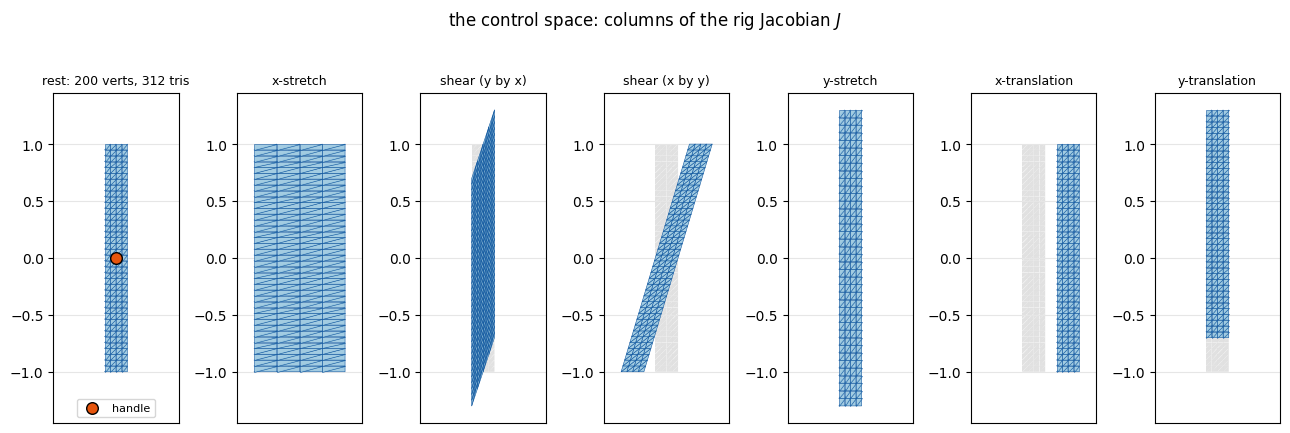
The simplest rig is a single affine handle: one LBS bone with weight 1 everywhere. simkit.lbs_jacobian
builds its Jacobian \(J\), the rig pose is \(x = J\,p\) with 6 parameters \(p\) (in 2D), and the columns of \(J\) span
every affine motion: the control space. p0 reproduces the rest shape, and handle_pose is the animator,
sweeping the handle’s \(x\)-translation \(p_{-2}\) back and forth.
def affine_rig(X):
    """One global affine LBS handle: its Jacobian J (x = J p) and the pose p0 with J p0 = X."""
    J = simkit.lbs_jacobian(X, np.ones((len(X), 1)))
    p0 = simkit.project_into_subspace(X.reshape(-1, 1), J)
    return J, p0

def handle_pose(p0, i):
    """The animator's input at step i: the rest pose with a sinusoidal x-translation."""
    p = p0.copy()
    p[-2] = AMP * np.sin(2 * np.pi * i / PERIOD)
    return p

J, p0 = affine_rig(X)
print(f"rig: J is {J.shape} -> {J.shape[1]} DOFs,  p0 = {np.round(p0.ravel(), 6)}")
rig: J is (400, 6) -> 6 DOFs, p0 = [ 1. 0. 0. 1. 0. -0.]
Left: the beam at rest and its handle (orange, at the translation origin). Right: each column of \(J\) applied to the beam over its gray rest shape. Any displacement in their span belongs to the animator.
col_names = ["x-stretch", "shear (y by x)", "shear (x by y)", "y-stretch", "x-translation", "y-translation"]
col_shapes = [X + MODE_SCALE * J[:, c].reshape(n, dim) / np.abs(J[:, c]).max() for c in range(J.shape[1])]
lims = utils.auto_limits([X] + col_shapes, pad=0.15)
fig, axes = plt.subplots(1, 7, figsize=(13, 4.8))
utils.plot_mesh(axes[0], X, T, title=f"rest: {n} verts, {len(T)} tris", lims=lims, lw=0.4)
axes[0].scatter(*p0[-2:].ravel(), s=70, color=utils.HANDLE_C, edgecolors="k", zorder=6, label="handle")
axes[0].legend(loc="lower center", fontsize=8)
for ax, shape, name in zip(axes[1:], col_shapes, col_names):
    utils.PolyMeshArtist(ax, X, T, facecolor="0.88", edgecolor="none", zorder=1)
    utils.plot_mesh(ax, shape, T, title=name, lims=lims, lw=0.4)
for ax in axes:
    ax.title.set_fontsize(9)
    ax.set_xticks([])
fig.suptitle("the control space: columns of the rig Jacobian $J$")
fig.tight_layout()
simkit.filesystem.save_figure(fig, os.path.join(RESULTS_DIR, "rig_modes.png"),
                              copy_to=os.path.join(MEDIA_DIR, "023_rig_modes.png"))
plt.show()
The animator’s input on its own: the handle (orange) sweeps left and right and the beam follows rigidly. There is no physics yet.
rig_states = [(J @ handle_pose(p0, i)).reshape(n, dim) for i in range(NSTEPS)]
handle_traj = [handle_pose(p0, i)[-2:].ravel() for i in range(NSTEPS)]
fig, anim = utils.animate_colored_mesh_panels(
    [dict(states=rig_states, T=T, title="rig pose  $x = J\\,p$", color=RIG_C, handle=handle_traj)],
    fps=FPS, suptitle="The animator's input: a rigid beam swept left and right")
video = simkit.filesystem.save_animation(anim, os.path.join(RESULTS_DIR, "rig.mp4"), fps=FPS, bitrate=BITRATE,
                                         copy_to=os.path.join(MEDIA_DIR, "023_rig.mp4"))
plt.close(fig)
utils.embed_video(video)
2 · Full-order complementary dynamics#
Each timestep is a backward-Euler step: minimize inertia plus ARAP elasticity over the total position \(x = J\,p_{\text{next}} + u_c\), with inertial target \(\tilde x = 2x_{\text{curr}} - x_{\text{prev}}\). The only thing that makes it complementary rather than ordinary elastodynamics is one linear constraint:
cd_operators precomputes everything constant: the mass matrix \(M\) (orthogonality is measured in momentum),
the deformation Jacobian \(G\) (positions to per-triangle \(F\)), the ARAP Laplacian \(L = G^\top W G\) with
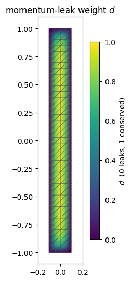
\(W = \mu\,\text{vol}\), the rig, and the momentum-leak field \(d\) (\(D = \operatorname{diag}(d)\)): diffuse 1
inward from the boundary and take one minus that. Where \(d = 0\) momentum leaks, so tissue rides along with the
rig; where \(d = 1\) it is conserved and resists. The constraint is \(A = J^\top M D\), and the constant KKT matrix
of the constrained global step (below) is factored once, here.
def cd_operators(X, T):
    """Constant operators of full-order complementary dynamics on the mesh (X, T)."""
    n, dim = X.shape
    M = sp.sparse.kron(simkit.massmatrix(X, T, rho=RHO), sp.sparse.eye(dim)).tocsc()
    G = simkit.deformation_jacobian(X, T)
    vol = simkit.volume(X, T)
    mu_s, lam_s = simkit.ympr_to_lame(YM, PR)
    mu = np.full((len(T), 1), mu_s)
    lam = np.full((len(T), 1), lam_s)
    W_arap = sp.sparse.kron(sp.sparse.diags((mu * vol).ravel()), sp.sparse.eye(dim * dim))
    L = (G.T @ W_arap @ G).tocsc()                                   # ARAP Laplacian (rotations frozen)
    J, p0 = affine_rig(X)
    bnd = np.unique(simkit.boundary_edges(T))
    leak = simkit.diffuse_field(X, T, bnd, np.ones((len(bnd), 1)), dt=LEAK_DT, normalize=True)
    d = 1.0 - leak
    D = sp.sparse.kron(sp.sparse.diags(d.ravel()), sp.sparse.eye(dim))
    A = J.T @ M @ D                                                  # rig-orthogonality constraint
    H_elastic = L                                                    # global-step matrix H = L + M / h^2
    H_inertia = M / DT**2
    H = (H_elastic + H_inertia).tocsc()
    A_sp = sp.sparse.csc_matrix(A)
    kkt_solve = sp.sparse.linalg.factorized(sp.sparse.bmat([[H, A_sp.T], [A_sp, None]]).tocsc())
    return dict(n=n, dim=dim, M=M, G=G, vol=vol, mu=mu, lam=lam, W_arap=W_arap, L=L,
                J=J, p0=p0, d=d, A=A, H=H, kkt_solve=kkt_solve)

ops = cd_operators(X, T)
print(f"constraint A = J^T M D: {ops['A'].shape},  KKT system: {ops['H'].shape[0] + ops['A'].shape[0]} unknowns")
constraint A = J^T M D: (6, 400), KKT system: 406 unknowns
The leak weight \(d\) is 0 on the whole surface of the thin beam (the diffusion seeds) and rises to 1 along its core, so the beam’s interior carries the momentum that will produce secondary motion.
fig, ax = plt.subplots(figsize=(3.4, 5.6))
utils.plot_scalar_field(ax, X, T, ops["d"], title="momentum-leak weight $d$", label="$d$  (0 leaks, 1 conserved)")
fig.tight_layout()
simkit.filesystem.save_figure(fig, os.path.join(RESULTS_DIR, "leak_field.png"),
                              copy_to=os.path.join(MEDIA_DIR, "023_leak_field.png"))
plt.show()
full_cd_system is one step’s objective in the complementary displacement \(u_c\). Its energy, gradient and
Hessian are inertia plus ARAP from simkit.energies (used below to validate the solver). The solver is block
coordinate descent (tutorials 21 and 22), so the system also returns its two steps: the local step fits the
closest rotation to each triangle’s \(F\) (polar_svd), and the global step freezes them and solves the
quadratic together with the constraint, the prefactored KKT system
\(\begin{bmatrix} H & A^{\top}\\ A & 0\end{bmatrix}\) with \(H = L + M/h^2\).
def full_cd_system(ops, u_curr, u_prev, p_curr, p_prev, p_next):
    """Backward-Euler step of full-order complementary dynamics, in the complementary displacement u."""
    n, dim, M, G, J, H = ops["n"], ops["dim"], ops["M"], ops["G"], ops["J"], ops["H"]
    mu, lam, vol, W_arap, kkt_solve = ops["mu"], ops["lam"], ops["vol"], ops["W_arap"], ops["kkt_solve"]
    n_con = ops["A"].shape[0]
    x_curr = J @ p_curr + u_curr
    x_prev = J @ p_prev + u_prev
    x_tilde = simkit.energies.be_target(x_curr, x_prev, DT)          # inertial target 2 x_curr - x_prev
    Jp = J @ p_next                                                  # the rig's pose this step

    def energy_func(u):
        x = Jp + u
        E_inertia = simkit.energies.kinetic_energy_be(x, x_curr, x_prev, M, DT)
        E_elastic = simkit.energies.elastic_energy_x(x.reshape(n, dim), G, mu, lam, vol, MATERIAL)
        E_total = E_inertia + E_elastic
        return E_total

    def gradient_func(u):
        x = Jp + u
        g_inertia = simkit.energies.kinetic_gradient_be(x, x_curr, x_prev, M, DT)
        g_elastic = simkit.energies.elastic_gradient_x(x.reshape(n, dim), G, mu, lam, vol, MATERIAL)
        g_total = g_inertia + g_elastic
        return g_total

    def hessian_func(u):
        x = Jp + u
        H_inertia = simkit.energies.kinetic_hessian_be(M, DT)
        H_elastic = simkit.energies.elastic_hessian_x(x.reshape(n, dim), G, mu, lam, vol, MATERIAL, psd=True)
        H_total = H_inertia + H_elastic
        return H_total

    def local_step(u):
        F = (G @ (Jp + u)).reshape(-1, dim, dim)
        R = simkit.polar_svd(F)[0]                                   # closest rotation, per triangle
        return R.reshape(-1, 1)

    def global_step(u, R):
        f_inertia = M @ x_tilde / DT**2
        f_elastic = G.T @ (W_arap @ R)
        f_rig = -H @ Jp
        f_total = f_inertia + f_elastic + f_rig
        return kkt_solve(np.vstack([f_total, np.zeros((n_con, 1))]))[: len(u)]

    return energy_func, gradient_func, hessian_func, local_step, global_step
rollout plays the animator’s sweep through either system: each step builds the system at the current state,
runs simkit.solvers.block_coord for BCD_ITERS local/global iterations, and records the pose \(J\,p + u_c\),
the rig-orthogonality residual \(\lVert J^{\top} M D\,u_c\rVert\) and the step’s wall-clock time. For the reduced
solver of section 3 the state is \(z\), lifted by its basis as \(u_c = B\,z\).
def rollout(system_func, ops, nsteps=NSTEPS):
    """Simulate the handle sweep; returns per-step poses, solver states, rig poses, residuals, seconds."""
    J, p0, A, dim = ops["J"], ops["p0"], ops["A"], ops["dim"]
    B = ops.get("B")                                                 # None for the full-order system
    s_curr = np.zeros((J.shape[0] if B is None else B.shape[1], 1))
    s_prev = s_curr.copy()
    p_curr, p_prev = p0.copy(), p0.copy()
    out = dict(states=[], s=[], p=[], residual=[], seconds=[])
    for i in range(nsteps):
        p_next = handle_pose(p0, i)
        t0 = time.perf_counter()
        _, _, _, local_step, global_step = system_func(ops, s_curr, s_prev, p_curr, p_prev, p_next)
        s_next = simkit.solvers.block_coord(s_curr, global_step, local_step, tolerance=0.0, max_iter=BCD_ITERS)
        out["seconds"].append(time.perf_counter() - t0)
        s_prev, s_curr = s_curr, s_next
        p_prev, p_curr = p_curr, p_next
        u_c = s_curr if B is None else B @ s_curr                    # complementary displacement
        out["states"].append((J @ p_curr + u_c).reshape(-1, dim))
        out["s"].append(s_curr)
        out["p"].append(p_curr)
        out["residual"].append(np.linalg.norm(A @ u_c))
    return out
Run the full-order solver under the sweep. The KKT solve holds the constraint to round-off at every step.
full = rollout(full_cd_system, ops)
t_full = 1000 * np.mean(full["seconds"])
print(f"full-order: {t_full:.1f} ms/step, {len(T)} rotations/step, {J.shape[0]} DOFs")
print(f"max rig-orthogonality residual  ||J^T M D u_c|| = {max(full['residual']):.1e}")
full-order: 5.8 ms/step, 312 rotations/step, 400 DOFs
max rig-orthogonality residual  ||J^T M D u_c|| = 1.0e-13
Top: the rig alone. Bottom: the same rig plus the complementary physics, over the rig pose in gray. The beam whips and trails as the handle reverses: secondary motion the animator never authored, and by construction none of it is a motion the handle could have made itself.
fig, anim = utils.animate_colored_mesh_panels([
    dict(states=rig_states, T=T, title="rig only  $J\\,p$", color=RIG_C, handle=handle_traj),
    dict(states=full["states"], T=T, title="rig + complementary  $J\\,p + u_c$", color=FULL_C,
         ghost=rig_states, handle=handle_traj),
], ncols=1, fps=FPS, suptitle="Full-order complementary dynamics")
video = simkit.filesystem.save_animation(anim, os.path.join(RESULTS_DIR, "full.mp4"), fps=FPS, bitrate=BITRATE,
                                         copy_to=os.path.join(MEDIA_DIR, "023_full.mp4"))
plt.close(fig)
utils.embed_video(video)
3 · Fast complementary dynamics#
The full step has two mesh-sized costs: a polar_svd for every triangle in each local step, and a sparse
KKT solve over every vertex in each global step. Refine the mesh and both grow. Fast complementary
dynamics removes both with two ideas.
Rig-orthogonal skinning eigenmodes. Restrict \(u_c = B\,z\) to skinning eigenmodes (tutorial 17) computed subject to \(J^\top M D\,B = 0\). The constraint then holds for any \(z\), and the global step is a tiny, unconstrained dense solve.
Rotation clustering. Triangles that move alike share one rotation per cluster in the local step.
fast_cd_operators precomputes both ideas. \(B\) = lbs_jacobian(X, W) is linear in the weight fields \(W\), so
\(J^\top M D\,B = 0\) is a linear constraint on each field \(w\); we assemble its rows with one einsum and pass an
SVD basis of them to skinning_eigenmodes(..., Aeq=...). (simkit.lbs_weight_space_constraint builds the same
rows, but its redundant-row removal keeps the first rows rather than an independent set, which for this rig
drops constraints.) spectral_cubature then clusters the triangles, and cluster_grouping_matrices gives the
cluster sums \(P\): the local step fits each cluster’s rotation to its \(\mu\,\text{vol}\)-weighted sum of \(F\).
def fast_cd_operators(X, T, ops):
    """Rig-orthogonal subspace B, rotation clusters and reduced matrices, added to the full operators."""
    n, dim, M, G, J, L, A = ops["n"], ops["dim"], ops["M"], ops["G"], ops["J"], ops["L"], ops["A"]
    # Idea 1: J^T M D B = 0 for B = lbs(W)  <=>  sum_v A[c, v, i] [X_v, 1]_j w[v] = 0 for every weight field w
    X1 = np.hstack([X, np.ones((n, 1))])
    C_w = np.einsum("cvi,vj->cijv", A.reshape(-1, n, dim), X1).reshape(-1, n)
    _, s_w, Vt_w = np.linalg.svd(C_w, full_matrices=False)
    Aeq = Vt_w[s_w > CONSTRAINT_RTOL * s_w[0]]                       # independent weight-space rows
    W, _, B = simkit.skinning_eigenmodes(X, T, K_MODES, Aeq=Aeq)
    B = simkit.orthonormalize(B, M=M)
    # Idea 2: cluster triangles; each cluster shares one rotation, fit to its (mu vol)-weighted sum of F
    _, _, labels = simkit.spectral_cubature(X, T, W, N_CLUSTERS, return_labels=True)
    labels = np.asarray(labels).ravel()
    P, _ = simkit.cluster_grouping_matrices(labels, X, T)
    P_w = sp.sparse.kron(P @ sp.sparse.diags((ops["mu"] * ops["vol"]).ravel()), sp.sparse.eye(dim * dim))
    GB = P_w @ G @ B                                                 # z -> clustered F sums
    GJ = P_w @ G @ J                                                 # p -> clustered F sums
    # reduced global-step matrices, factored once
    BMB = B.T @ M @ B
    BMJ = B.T @ M @ J
    BLJ = B.T @ L @ J
    H_red_elastic = B.T @ L @ B
    H_red_inertia = BMB / DT**2
    H_red = H_red_elastic + H_red_inertia
    chol = sp.linalg.cho_factor(H_red)
    return dict(ops, Aeq=Aeq, W=W, B=B, labels=labels, n_clusters=P.shape[0],
                GB=GB, GJ=GJ, BMB=BMB, BMJ=BMJ, BLJ=BLJ, chol=chol)

red_ops = fast_cd_operators(X, T, ops)
print(f"weight-space constraint: {red_ops['Aeq'].shape},  subspace B: {red_ops['B'].shape}")
print(f"structural rig-orthogonality  ||(J^T M D) B|| = {np.linalg.norm(ops['A'] @ red_ops['B']):.1e}")
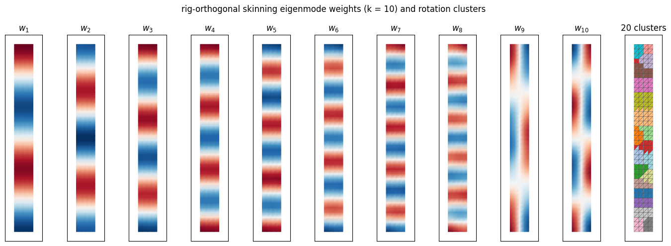
weight-space constraint: (6, 200),  subspace B: (400, 60)
structural rig-orthogonality  ||(J^T M D) B|| = 2.2e-12
The printout confirms 6 independent constraint rows and a 60-column \(B\) that is rig-orthogonal to round-off. Below, its weight fields \(w_k\) (red and blue are opposite signs; each field spawns 6 columns of \(B\)) and the rotation clusters, one color per shared rotation: 20 clusters capture the whole beam’s bending, so the local step’s cost no longer depends on how finely it is meshed.
fig, axes = plt.subplots(1, K_MODES + 1, figsize=(14, 5.0))
for k, ax in enumerate(axes[:-1]):
    w = red_ops["W"][:, k]
    vmax = np.abs(w).max()
    utils.plot_scalar_field(ax, X, T, w, title=f"$w_{{{k + 1}}}$", cmap="RdBu_r", vmin=-vmax, vmax=vmax,
                            edges=False, colorbar=False)
utils.plot_scalar_field(axes[-1], X, T, red_ops["labels"], title=f"{red_ops['n_clusters']} clusters",
                        cmap="tab20", edges=True, colorbar=False)
for ax in axes:
    ax.set_xticks([])
    ax.set_yticks([])
fig.suptitle(f"rig-orthogonal skinning eigenmode weights (k = {K_MODES}) and rotation clusters")
fig.tight_layout()
simkit.filesystem.save_figure(fig, os.path.join(RESULTS_DIR, "subspace.png"),
                              copy_to=os.path.join(MEDIA_DIR, "023_subspace.png"))
plt.show()
fast_cd_system mirrors full_cd_system in subspace coordinates \(z\). Its energy, gradient and Hessian are the
same inertia plus ARAP at \(x = J\,p_{\text{next}} + B\,z\), pulled back by \(B^\top\) (per-triangle rotations, the
reference the clustered solver approximates). The local step is one polar_svd per cluster, and the global step
solves the dense reduced system \((B^\top L B + B^\top M B/h^2)\,z = f\) with the prefactored Cholesky factor.
def fast_cd_system(ops, z_curr, z_prev, p_curr, p_prev, p_next):
    """Backward-Euler step of fast complementary dynamics, in the rig-orthogonal subspace coordinates z."""
    n, dim, M, G, J, B = ops["n"], ops["dim"], ops["M"], ops["G"], ops["J"], ops["B"]
    mu, lam, vol = ops["mu"], ops["lam"], ops["vol"]
    GB, GJ, BMB, BMJ, BLJ, chol = ops["GB"], ops["GJ"], ops["BMB"], ops["BMJ"], ops["BLJ"], ops["chol"]
    x_curr = J @ p_curr + B @ z_curr
    x_prev = J @ p_prev + B @ z_prev
    z_tilde = simkit.energies.be_target(z_curr, z_prev, DT)          # inertial targets in z and p
    p_tilde = simkit.energies.be_target(p_curr, p_prev, DT)
    Jp = J @ p_next

    def energy_func(z):
        x = Jp + B @ z
        E_inertia = simkit.energies.kinetic_energy_be(x, x_curr, x_prev, M, DT)
        E_elastic = simkit.energies.elastic_energy_x(x.reshape(n, dim), G, mu, lam, vol, MATERIAL)
        E_total = E_inertia + E_elastic
        return E_total

    def gradient_func(z):
        x = Jp + B @ z
        g_inertia = B.T @ simkit.energies.kinetic_gradient_be(x, x_curr, x_prev, M, DT)
        g_elastic = B.T @ simkit.energies.elastic_gradient_x(x.reshape(n, dim), G, mu, lam, vol, MATERIAL)
        g_total = g_inertia + g_elastic
        return g_total

    def hessian_func(z):
        x = Jp + B @ z
        H_inertia = B.T @ (simkit.energies.kinetic_hessian_be(M, DT) @ B)
        H_elastic = B.T @ (simkit.energies.elastic_hessian_x(x.reshape(n, dim), G, mu, lam, vol, MATERIAL,
                                                             psd=True) @ B)
        H_total = H_inertia + H_elastic
        return H_total

    def local_step(z):
        F_c = (GB @ z + GJ @ p_next).reshape(-1, dim, dim)
        R_c = simkit.polar_svd(F_c)[0]                               # one rotation per cluster
        return R_c.reshape(-1, 1)

    def global_step(z, R_c):
        f_inertia = BMB @ z_tilde / DT**2
        f_rig_inertia = -BMJ @ (p_next - p_tilde) / DT**2
        f_elastic = GB.T @ R_c
        f_rig_elastic = -BLJ @ p_next
        f_total = f_inertia + f_rig_inertia + f_elastic + f_rig_elastic
        return sp.linalg.cho_solve(chol, f_total)

    return energy_func, gradient_func, hessian_func, local_step, global_step
Run the fast solver under the same sweep. It is several times faster already on this small mesh, and keeps the residual at round-off without any constraint solve.
red = rollout(fast_cd_system, red_ops)
t_red = 1000 * np.mean(red["seconds"])
print(f"reduced: {t_red:.2f} ms/step, {red_ops['n_clusters']} rotations/step, {red_ops['B'].shape[1]} DOFs"
      f"   ->   {t_full / t_red:.1f}x faster than full-order")
print(f"max rig-orthogonality residual  ||J^T M D B z|| = {max(red['residual']):.1e}")
reduced: 0.73 ms/step, 20 rotations/step, 60 DOFs   ->   8.0x faster than full-order
max rig-orthogonality residual  ||J^T M D B z|| = 3.7e-13
4 · Validating both solvers#
Three cheap checks at step VALID_STEP: each system’s gradient against central differences (simkit.gradient_cfd),
the energy per local/global iteration, and the rig-orthogonality residual over the whole run. For the reduced
system, Newton on the same subspace energy with per-triangle rotations (its hessian_func) gives the minimum that
rotation clustering trades away.
i = VALID_STEP
fig, axes = plt.subplots(1, 3, figsize=(15, 4.3))
curves = {}
for name, system_func, sys_ops, run, color in [("full-order", full_cd_system, ops, full, FULL_C),
                                                ("fast (reduced)", fast_cd_system, red_ops, red, RED_C)]:
    energy_func, gradient_func, hessian_func, local_step, global_step = system_func(
        sys_ops, run["s"][i], run["s"][i - 1], run["p"][i], run["p"][i - 1], handle_pose(p0, i + 1))
    s0 = run["s"][i]
    g = gradient_func(s0).ravel()
    g_fd = simkit.gradient_cfd(lambda s: np.array(energy_func(s.reshape(-1, 1))), s0.ravel().copy(), FD_H)
    print(f"{name:15s} gradient vs central differences: relative error {np.linalg.norm(g_fd - g) / np.linalg.norm(g):.1e}")
    axes[0].plot(g_fd, g, "o", ms=3, color=color, label=name)
    s, energies = s0.copy(), [energy_func(s0)]
    for _ in range(VALID_ITERS):
        s = global_step(s, local_step(s))
        energies.append(energy_func(s))
    curves[name] = np.array(energies) - energies[-1]
    if system_func is fast_cd_system:
        s_newton = simkit.solvers.newton_solver(s0.copy(), energy_func, gradient_func, hessian_func,
                                                max_iter=NEWTON_ITERS, tolerance=NEWTON_TOL)
        E_bcd, E_newton = energies[BCD_ITERS], energy_func(s_newton)
        print(f"{name:15s} energy after {BCD_ITERS} clustered BCD iterations {E_bcd:.2f}  vs  Newton with per-triangle "
              f"rotations {E_newton:.2f}  (+{100 * (E_bcd - E_newton) / E_newton:.1f}%)")
lo, hi = axes[0].get_xlim()
axes[0].plot([lo, hi], [lo, hi], "k--", lw=1, label="analytic = FD")
axes[0].set_xlabel("central-difference gradient entry")
axes[0].set_ylabel("analytic gradient entry")
axes[0].set_title("gradient check")
axes[0].legend(fontsize=9)
axes[0].grid(True, color="0.9")
utils.residual_plot(curves, ax=axes[1], colors={"full-order": FULL_C, "fast (reduced)": RED_C}, markers=True,
                    xlabel="local/global iteration", ylabel="$E_k - E_{%d}$" % VALID_ITERS,
                    title="block coordinate descent decreases the energy")
axes[1].axvline(BCD_ITERS, color="0.5", ls=":", lw=1.2)
utils.residual_plot({"full-order": full["residual"][1:], "fast (reduced)": red["residual"][1:]},
                    np.arange(1, NSTEPS), ax=axes[2], colors={"full-order": FULL_C, "fast (reduced)": RED_C},
                    ylim=(1e-16, 1e-10), xlabel="step", ylabel="$\\|\\,J^\\top M D\\,u_c\\,\\|$",
                    title="rig-orthogonality residual (steps 1+)")
fig.tight_layout()
simkit.filesystem.save_figure(fig, os.path.join(RESULTS_DIR, "validation.png"),
                              copy_to=os.path.join(MEDIA_DIR, "023_validation.png"))
plt.show()
full-order      gradient vs central differences: relative error 3.3e-10
fast (reduced)  gradient vs central differences: relative error 1.0e-09
fast (reduced)  energy after 10 clustered BCD iterations 1486.93  vs  Newton with per-triangle rotations 1478.48  (+0.6%)
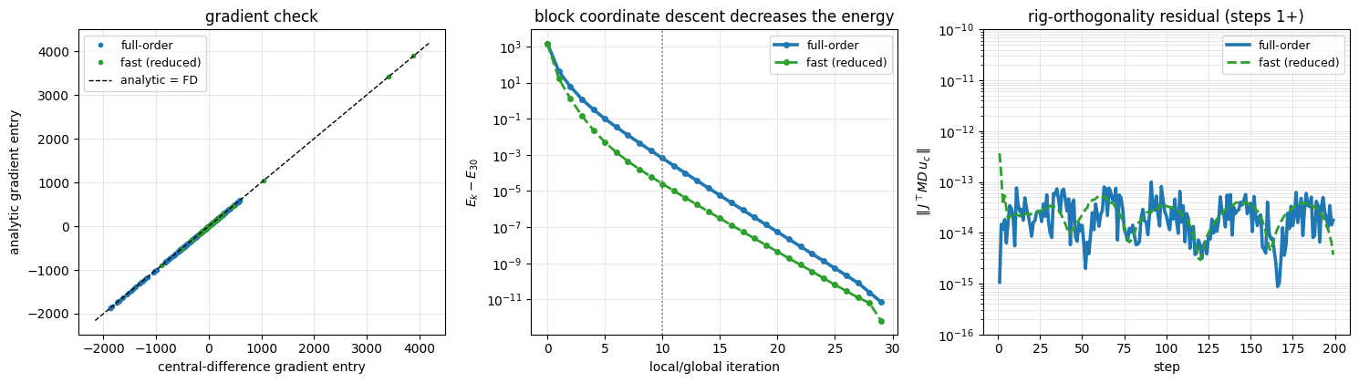
The analytic gradients sit on the diagonal. Both solvers decrease the energy at every local/global iteration
(dotted line: the BCD_ITERS used per step), and the residual stays at round-off throughout: enforced by the
KKT solve in the full model, structural in the reduced one. Clustering is cheap in accuracy too: the clustered
solve ends only 0.6% above the per-triangle-rotation minimum of the same subspace.
5 · Rig vs. full vs. reduced#
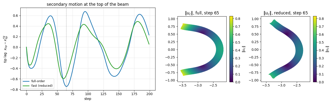
The reduced solve reproduces the full-order secondary motion (the same whip and trail) while solving a 60-DOF dense system with 20 rotations instead of a 406-unknown KKT system with 312.
fig, anim = utils.animate_colored_mesh_panels([
    dict(states=rig_states, T=T, title="rig", color=RIG_C, handle=handle_traj),
    dict(states=full["states"], T=T, title=f"full  ({len(T)} rotations, {J.shape[0]} DOFs)", color=FULL_C,
         ghost=rig_states, handle=handle_traj),
    dict(states=red["states"], T=T, title=f"reduced  ({red_ops['n_clusters']} rotations, {red_ops['B'].shape[1]} DOFs)",
         color=RED_C, ghost=rig_states, handle=handle_traj),
], ncols=1, fps=FPS, suptitle="Complementary dynamics: full-order vs. fast (skinning eigenmodes)")
video = simkit.filesystem.save_animation(anim, os.path.join(RESULTS_DIR, "compare.mp4"), fps=FPS, bitrate=BITRATE,
                                         copy_to=os.path.join(MEDIA_DIR, "023_compare.mp4"))
plt.close(fig)
utils.embed_video(video)
Quantitatively: the horizontal lag of the beam’s top vertex behind the rig, and the complementary displacement magnitude \(\lVert u_c\rVert\) at the step of largest lag (dotted), on the deformed beams with one shared color scale. The reduced tip swings in phase with the full one at a somewhat smaller amplitude: 60 DOFs and 20 shared rotations make the beam a little stiffer, but the displacement pattern (largest at the tips) is the same.
tip = np.argmin(np.linalg.norm(X - np.array([0.0, X[:, 1].max()]), axis=1))
lag = {name: np.array([s[tip, 0] - r[tip, 0] for s, r in zip(run["states"], rig_states)])
       for name, run in [("full-order", full), ("fast (reduced)", red)]}
i_max = int(np.argmax(np.abs(lag["full-order"])))
uc_mag = {name: np.linalg.norm(run["states"][i_max] - rig_states[i_max], axis=1) for name, run in [("full", full), ("reduced", red)]}
vmax = max(v.max() for v in uc_mag.values())
lims = utils.auto_limits([full["states"][i_max], red["states"][i_max]], pad=0.1)
fig, axes = plt.subplots(1, 3, figsize=(14, 4.4), gridspec_kw={"width_ratios": [2.2, 1, 1]})
utils.line_plot(np.arange(NSTEPS), lag, colors={"full-order": FULL_C, "fast (reduced)": RED_C}, ax=axes[0],
                xlabel="step", ylabel="tip lag  $x_{tip} - x_{tip}^{rig}$", title="secondary motion at the top of the beam")
axes[0].axvline(i_max, color="0.5", ls=":", lw=1.2)
for ax, (name, run) in zip(axes[1:], [("full", full), ("reduced", red)]):
    utils.plot_scalar_field(ax, run["states"][i_max], T, uc_mag[name], title=f"$\\|u_c\\|$, {name}, step {i_max}",
                            vmin=0, vmax=vmax, lims=lims, edges=False, label="$\\|u_c\\|$")
fig.tight_layout()
simkit.filesystem.save_figure(fig, os.path.join(RESULTS_DIR, "secondary_motion.png"),
                              copy_to=os.path.join(MEDIA_DIR, "023_secondary_motion.png"))
plt.show()
6 · Timing: how the gap grows with resolution#
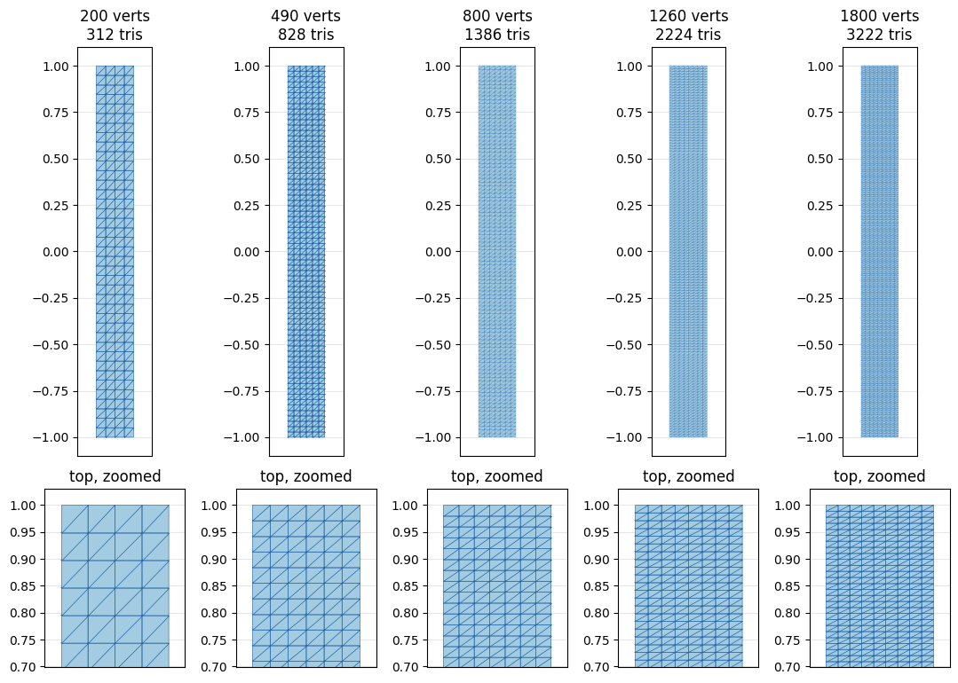
The reduced cost is set by the subspace size and the cluster count, both fixed as the mesh is refined, while the full-order cost grows with it. We sweep these beam meshes (bottom row: the top of each beam, zoomed), all with the same rig, leak-field construction and subspace sizes.
sweep_meshes = [beam_mesh(nx, ny) for nx, ny in SWEEP_RES]
fig, axes = plt.subplots(2, len(sweep_meshes), figsize=(11, 7.8), gridspec_kw={"height_ratios": [2.3, 1]})
for (ax, ax_zoom), (Xs, Ts) in zip(axes.T, sweep_meshes):
    utils.plot_mesh(ax, Xs, Ts, title=f"{len(Xs)} verts\n{len(Ts)} tris", lw=0.15 if len(Xs) > 500 else 0.4)
    utils.plot_mesh(ax_zoom, Xs, Ts, title="top, zoomed", lims=((-0.13, 0.13), (0.7, 1.03)), lw=0.4)
    ax.set_xticks([])
    ax_zoom.set_xticks([])
fig.tight_layout()
simkit.filesystem.save_figure(fig, os.path.join(RESULTS_DIR, "sweep_meshes.png"),
                              copy_to=os.path.join(MEDIA_DIR, "023_sweep_meshes.png"))
plt.show()
At each resolution we build both solvers and take the median cost of BENCH_STEPS steps after BENCH_WARMUP
untimed ones.
verts, t_fulls, t_reds = [], [], []
for Xs, Ts in sweep_meshes:
    ops_s = cd_operators(Xs, Ts)
    red_ops_s = fast_cd_operators(Xs, Ts, ops_s)
    tf = 1000 * np.median(rollout(full_cd_system, ops_s, BENCH_WARMUP + BENCH_STEPS)["seconds"][BENCH_WARMUP:])
    tr = 1000 * np.median(rollout(fast_cd_system, red_ops_s, BENCH_WARMUP + BENCH_STEPS)["seconds"][BENCH_WARMUP:])
    verts.append(len(Xs))
    t_fulls.append(tf)
    t_reds.append(tr)
    print(f"{len(Xs):5d} verts / {len(Ts):5d} tris:  full {tf:6.1f} ms   reduced {tr:5.2f} ms   ({tf / tr:5.1f}x)")

fig, (axL, axR) = plt.subplots(1, 2, figsize=(13, 4.2))
utils.line_plot(verts, {"full-order": t_fulls, "fast (reduced)": t_reds}, xlabel="vertices", ylabel="ms / step",
                markers=True, logy=True, colors={"full-order": FULL_C, "fast (reduced)": RED_C}, ax=axL,
                title="per-step cost")
utils.line_plot(verts, {"speedup": np.array(t_fulls) / np.array(t_reds)}, xlabel="vertices",
                ylabel="speedup  (full / reduced)", markers=True, colors={"speedup": "0.2"}, ax=axR,
                title="speedup grows with resolution")
fig.tight_layout()
simkit.filesystem.save_figure(fig, os.path.join(RESULTS_DIR, "timing.png"),
                              copy_to=os.path.join(MEDIA_DIR, "023_timing.png"))
plt.show()
200 verts / 312 tris: full 5.4 ms reduced 0.67 ms ( 8.1x)
490 verts / 828 tris: full 13.2 ms reduced 0.67 ms ( 19.6x)
800 verts / 1386 tris: full 22.1 ms reduced 0.70 ms ( 31.6x)
1260 verts / 2224 tris: full 34.4 ms reduced 0.69 ms ( 49.8x)
1800 verts / 3222 tris: full 50.0 ms reduced 0.71 ms ( 70.9x)
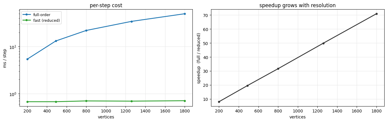
The full-order cost climbs with the vertex count while the reduced cost stays flat, so the speedup widens with every refinement.
Takeaways#
Complementary dynamics is ordinary elastodynamics plus one constraint, \(J^{\top} M D\,u_c = 0\): the secondary motion may carry no momentum the rig accounts for, and the leak field \(D\) picks where tissue rides with the rig.
Full order enforces it explicitly with a KKT global step inside ARAP block coordinate descent: correct, but both the per-triangle rotations and the KKT solve scale with the mesh.
Fast complementary dynamics moves both costs off the mesh: rig-orthogonal skinning eigenmodes make the constraint structural (a tiny unconstrained dense solve), and rotation clustering fixes the number of rotations.
Apart from the one-line weight-space constraint, every ingredient is a
simkitcall:lbs_jacobian,diffuse_field,skinning_eigenmodes,spectral_cubature,cluster_grouping_matrices,polar_svd,solvers.block_coordand the energies in each*_system.