0 · Discretizing a Deformation — the Finite Element Method#
Here is a smooth, recognizable shape. Suppose we ask the most basic question in all of solid mechanics:
how does this shape deform?
To answer it we need, at every material point \(\bar x\) of the rest shape, a displacement telling us where that point goes. Collecting all of those displacements gives a deformation map
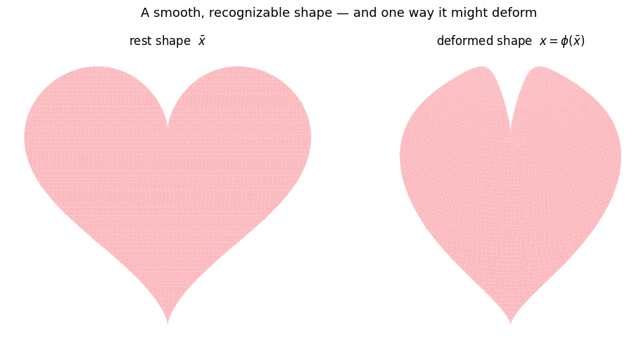
where \(u(\bar x)\) is the displacement field. The picture below shows the rest shape and one possible deformed shape — both drawn as smooth, continuous blobs (no triangles in sight… yet).
This first tutorial is about a single, foundational idea: a computer cannot store \(u\) at infinitely many points, so we have to discretize it. The finite element method (FEM) is the classic way to do that for elastic PDEs, and everything in the tutorials that follow is built on top of it.
%matplotlib inline
import numpy as np
import matplotlib.pyplot as plt
import matplotlib.tri as mtri
from matplotlib.collections import PolyCollection
from matplotlib.patches import Polygon
from matplotlib.path import Path
from matplotlib.animation import FuncAnimation
from scipy.spatial import Delaunay        # a general triangulator -- NOT a mesh file, NOT igl
import simkit
import utils

HEART_FACE = "#fbb4b9"    # soft pink fill
HEART_EDGE = "#c51b8a"    # magenta edges / arrows
A shape we build ourselves#
No mesh files here: we define the shape analytically with the classic heart curve
and then build a triangle mesh for its interior ourselves with a generic
Delaunay triangulator (no meshing library, no igl): scatter points inside the
outline, triangulate them, and throw away any triangle whose centre falls
outside the heart.
For the deformation we pick something simple and recognizable: a gentle bend that curls the heart about its vertical axis. It is an analytic map \(\phi\) — we can evaluate the true displacement \(u(\bar x) = \phi(\bar x) - \bar x\) at any point we like. That is exactly the luxury a computer does not have.
def heart_outline(n):
    """n points around the analytic heart curve, normalized into [-1, 1]^2."""
    t = np.linspace(0.0, 2.0 * np.pi, n, endpoint=False)
    x = 16.0 * np.sin(t) ** 3
    y = 13.0 * np.cos(t) - 5.0 * np.cos(2 * t) - 2.0 * np.cos(3 * t) - np.cos(4 * t)
    P = np.column_stack([x, y]).astype(float)
    P -= 0.5 * (P.max(0) + P.min(0))          # centre the bounding box at the origin
    P /= np.abs(P).max()                       # scale into [-1, 1]
    return P

def triangulate_heart(n_boundary, spacing):
    """A triangle mesh of the heart's interior, built with Delaunay + a point-in-shape test."""
    B = heart_outline(n_boundary)
    region = Path(B)
    g = np.arange(-1.0, 1.0 + 1e-9, spacing)            # a grid of candidate interior points
    XX, YY = np.meshgrid(g, g)
    P = np.column_stack([XX.ravel(), YY.ravel()])
    jit = np.linspace(0.0, 1.0, len(P))                 # tiny deterministic jitter -> nicer triangles
    P = P + (spacing * 0.18) * np.column_stack([np.sin(53 * jit), np.cos(37 * jit)])
    P = P[region.contains_points(P, radius=-0.45 * spacing)]   # keep points safely inside
    pts = np.vstack([B, P])
    F = Delaunay(pts).simplices
    F = F[region.contains_points(pts[F].mean(1))]       # drop triangles outside the heart
    return pts, F

# A simple, recognizable deformation  phi(x) = x + u(x):  bend about the vertical axis x = 0.
def deform(P, k=0.7):
    """The TRUE smooth deformation map phi, evaluable at any points P. Curvature k."""
    P = np.asarray(P, float)
    if abs(k) < 1e-9:
        return P.copy()
    R = 1.0 / k
    s = P[:, 0]               # position along the bending axis (heart is centred at x=0)
    h = P[:, 1]               # height above the axis
    theta = s / R             # bend angle grows with arc length
    r = R - h
    return np.column_stack([r * np.sin(theta), R - r * np.cos(theta)])

def show_shape(ax, U, Tris, *, edges=False, title="", face=HEART_FACE, lw=0.5):
    """Fill a triangle mesh. With edges=False it looks like a smooth continuous blob."""
    ec = HEART_EDGE if edges else "none"
    ax.add_collection(PolyCollection([U[f] for f in Tris], facecolors=face,
                                     edgecolors=ec, linewidths=(lw if edges else 0.0),
                                     alpha=0.95))
    ax.set_aspect("equal"); ax.autoscale(); ax.margins(0.06); ax.axis("off")
    if title:
        ax.set_title(title, fontsize=12)

X, T = triangulate_heart(n_boundary=360, spacing=0.028)    # a fine mesh for the smooth look
print(f"a smooth heart: {X.shape[0]} points, {T.shape[0]} triangles")

fig, axes = plt.subplots(1, 2, figsize=(10, 5))
show_shape(axes[0], X, T, title=r"rest shape  $\bar{x}$")
show_shape(axes[1], deform(X), T, title=r"deformed shape  $x = \phi(\bar{x})$")
fig.suptitle("A smooth, recognizable shape — and one way it might deform", fontsize=13)
fig.tight_layout(); fig.savefig("media/00_teaser.png", dpi=130, bbox_inches="tight")
plt.show()
a smooth heart: 3238 points, 6026 triangles
The deformation is a vector field#
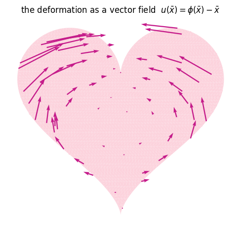
The deformation map carries one piece of information at every point: a little arrow \(u(\bar x)\) saying which way, and how far, that material point moves. Drawing those arrows on the rest shape gives the displacement vector field. Near the bottom tip the arrows are tiny (that part barely moves); up at the lobes they sweep inward and up as the heart curls.
Finding this field \(u\) — one arrow per point — is the problem we want to solve.
U_def = deform(X)
disp = U_def - X
idx = np.arange(0, X.shape[0], 55)          # subsample so the arrows are readable

fig, ax = plt.subplots(figsize=(6.5, 5.5))
show_shape(ax, X, T, face="#fcd0db",
           title=r"the deformation as a vector field  $u(\bar{x}) = \phi(\bar{x}) - \bar{x}$")
ax.quiver(X[idx, 0], X[idx, 1], disp[idx, 0], disp[idx, 1], angles="xy",
          scale_units="xy", scale=1, color=HEART_EDGE, width=0.005, zorder=5)
fig.savefig("media/00_field.png", dpi=130, bbox_inches="tight")
plt.show()
# Watch the field "push" the shape from rest to deformed (the arrows grow with it).
frames = 36
ts = 0.5 * (1 - np.cos(np.linspace(0, np.pi, frames)))   # smooth ease 0 -> 1
states = [X + t * disp for t in ts]
(xlim, ylim) = utils.auto_limits(states, pad=0.12)

fig, ax = plt.subplots(figsize=(6.5, 5.5))
ax.set_aspect("equal"); ax.set_xlim(*xlim); ax.set_ylim(*ylim); ax.axis("off")
ax.set_title("the field carries every point from rest to deformed", fontsize=12)
mesh = utils.PolyMeshArtist(ax, states[0], T, facecolor=HEART_FACE, edgecolor="none")
q = ax.quiver(X[idx, 0], X[idx, 1], 0 * disp[idx, 0], 0 * disp[idx, 1], angles="xy",
              scale_units="xy", scale=1, color=HEART_EDGE, width=0.005, zorder=5)

def update(i):
    mesh.update(states[i])
    q.set_UVC(ts[i] * disp[idx, 0], ts[i] * disp[idx, 1])
    return ()

anim = FuncAnimation(fig, update, frames=frames, interval=1000 / 20, blit=False)
utils.show_video(fig, anim, "media/00_morph.mp4", fps=20)
The catch: there are infinitely many points#
A smooth shape has a continuum of material points. We cannot ask a computer to find \(u(\bar x)\) at infinitely many \(\bar x\) — we need a finite list of unknowns.
This is what the finite element method does, and the idea is wonderfully simple:
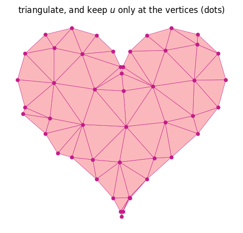
Triangulate the shape into a mesh of triangles (the elements).
Store the displacement \(u\) only at the vertices — a finite set of unknowns.
To get \(u\) anywhere else, interpolate the surrounding vertex values across the triangle.
So the whole continuous field collapses down to a handful of arrows, one per vertex. Everything in between is reconstructed by interpolation.
# A deliberately COARSE mesh of the same heart, so the elements are big and visible.
Xc, Tc = triangulate_heart(n_boundary=28, spacing=0.34)
print(f"coarse FEM mesh: {Xc.shape[0]} vertices, {Tc.shape[0]} triangles")
print("we will only ever solve for u at those vertices.")

fig, ax = plt.subplots(figsize=(6.5, 5.5))
show_shape(ax, Xc, Tc, edges=True,
           title="triangulate, and keep $u$ only at the vertices (dots)")
used = np.unique(Tc)                                   # only vertices that belong to a triangle
ax.scatter(Xc[used, 0], Xc[used, 1], s=22, color=HEART_EDGE, zorder=6)
fig.savefig("media/00_mesh.png", dpi=130, bbox_inches="tight")
plt.show()
coarse FEM mesh: 50 vertices, 64 triangles
we will only ever solve for u at those vertices.
Inside one triangle: barycentric interpolation#
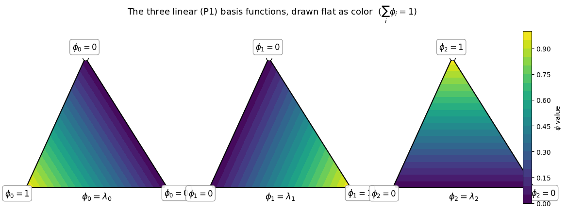
How do we reconstruct \(u\) inside a triangle from its three corner values? Every point \(\bar x\) in a triangle with corners \(\bar x_0, \bar x_1, \bar x_2\) has a unique set of barycentric coordinates \((\lambda_0, \lambda_1, \lambda_2)\) with
The \(\lambda_i\) are also the linear (P1) basis functions \(\phi_i\) of the triangle. Each one equals \(1\) at its own vertex, \(0\) at the other two, and varies linearly in between. Below each \(\phi_i\) is drawn flat, as a color over the triangle (bright \(= 1\) at its vertex, dark \(= 0\) at the others).
def barycentric(p, V):
    """Barycentric coords (lambda0, lambda1, lambda2) of point p in triangle V (3x2)."""
    M = np.array([[V[0, 0] - V[2, 0], V[1, 0] - V[2, 0]],
                  [V[0, 1] - V[2, 1], V[1, 1] - V[2, 1]]])
    a, b = np.linalg.solve(M, np.asarray(p, float) - V[2])
    return np.array([a, b, 1.0 - a - b])

# A single triangle, finely sampled inside; color each point by phi_i = lambda_i.
Vtri = np.array([[0.0, 0.0], [1.0, 0.0], [0.42, 0.92]])
m = 80
pts, lam = [], []
for i in range(m + 1):
    for j in range(m + 1 - i):
        a, b = i / m, j / m
        c = 1.0 - a - b
        pts.append(a * Vtri[0] + b * Vtri[1] + c * Vtri[2])
        lam.append((a, b, c))
pts = np.array(pts); lam = np.array(lam)
tri = mtri.Triangulation(pts[:, 0], pts[:, 1])
centroid = Vtri.mean(0)

fig, axes = plt.subplots(1, 3, figsize=(13.5, 4.6))
for k in range(3):
    ax = axes[k]
    tcf = ax.tricontourf(tri, lam[:, k], levels=np.linspace(0, 1, 21), cmap="viridis")
    ax.plot([Vtri[0, 0], Vtri[1, 0], Vtri[2, 0], Vtri[0, 0]],
            [Vtri[0, 1], Vtri[1, 1], Vtri[2, 1], Vtri[0, 1]], "k", lw=1.5)
    for v in range(3):                                  # value label, nudged outward from the centre
        d = Vtri[v] - centroid; d = d / np.linalg.norm(d)
        ax.scatter(*Vtri[v], s=70, color="white", edgecolor="k", zorder=5)
        ax.annotate(rf"$\phi_{k}={1 if v == k else 0}$", Vtri[v], textcoords="offset points",
                    xytext=(16 * d[0], 16 * d[1]), ha="center", va="center", fontsize=12, zorder=6,
                    bbox=dict(boxstyle="round", fc="white", ec="0.6", alpha=0.9))
    ax.set_title(rf"$\phi_{k} = \lambda_{k}$", y=-0.12, fontsize=13)
    ax.set_aspect("equal"); ax.axis("off"); ax.margins(0.22)
cb = fig.colorbar(tcf, ax=axes, fraction=0.022, pad=0.06); cb.set_label(r"$\phi$ value")
fig.suptitle(r"The three linear (P1) basis functions, drawn flat as color  ($\sum_i \phi_i = 1$)",
             fontsize=13, y=1.0)
fig.subplots_adjust(top=0.84, bottom=0.1, wspace=0.3)
fig.savefig("media/00_hats.png", dpi=130, bbox_inches="tight")
plt.show()
Combining the hats into a vector interpolation#
Now give each corner its own displacement vector \(u_0, u_1, u_2\). The displacement at any interior point is the basis-weighted blend
So the value at the three vertices is all we store; the arrow everywhere else is reconstructed from them. Watch the evaluation point (orange) sweep across the triangle: its arrow continuously rebalances between the three corner arrows (blue), and as it approaches a vertex, \(\lambda\) collapses onto that vertex and the interpolated arrow matches the vertex’s own arrow exactly.
Vtri = np.array([[0.0, 0.0], [1.7, 0.15], [0.65, 1.45]])     # a generic triangle
Uv   = np.array([[0.28, -0.30], [0.42, 0.22], [-0.18, 0.46]])  # one vector per corner

# A path (in barycentric weights) that lingers near each corner, then the centre.
key = np.array([[0.34, 0.33, 0.33],
                [0.86, 0.07, 0.07],     # near corner 0
                [0.34, 0.33, 0.33],
                [0.07, 0.86, 0.07],     # near corner 1
                [0.34, 0.33, 0.33],
                [0.07, 0.07, 0.86],     # near corner 2
                [0.34, 0.33, 0.33]])
seg = 26
path_bary = np.vstack([np.linspace(key[i], key[i + 1], seg, endpoint=False)
                       for i in range(len(key) - 1)])
path_xy = path_bary @ Vtri                                     # the moving point x

fig, ax = plt.subplots(figsize=(6.6, 6.0))
ax.add_patch(Polygon(Vtri, closed=True, facecolor=utils.TRI_FACE,
                     edgecolor=utils.TRI_EDGE, lw=2.5, alpha=0.55, zorder=1))
for i in range(3):                                             # the fixed corner arrows
    ax.quiver(Vtri[i, 0], Vtri[i, 1], Uv[i, 0], Uv[i, 1], angles="xy",
              scale_units="xy", scale=1, color=utils.PIN_C, width=0.012, zorder=4)
    ax.scatter(*Vtri[i], s=90, color=utils.TRI_EDGE, zorder=5)
    ax.annotate(rf"$u_{i}$", Vtri[i] + np.array([0.04, 0.04]), fontsize=13,
                color=utils.PIN_C)
ax.set_aspect("equal"); ax.autoscale(); ax.margins(0.32); ax.axis("off")

q_pt = ax.quiver(path_xy[0, 0], path_xy[0, 1], 0, 0, angles="xy", scale_units="xy",
                 scale=1, color=utils.HANDLE_C, width=0.015, zorder=7)
dot, = ax.plot([], [], "o", color=utils.HANDLE_C, ms=9, zorder=8)
txt = ax.text(0.02, 1.1, "", transform=ax.transAxes, va="top", family="monospace",
              fontsize=11, bbox=dict(boxstyle="round", fc="white", ec="0.6", alpha=0.9))

def update(i):
    p = path_xy[i]
    lam = barycentric(p, Vtri)            # recovered from the position alone
    u = lam @ Uv                          # u(x) = sum lambda_i u_i
    q_pt.set_offsets(p); q_pt.set_UVC(u[0], u[1])
    dot.set_data([p[0]], [p[1]])
    txt.set_text(f"lambda = ({lam[0]:.2f}, {lam[1]:.2f}, {lam[2]:.2f})\n"
                 f"u(x)   = {lam[0]:.2f} u0 + {lam[1]:.2f} u1 + {lam[2]:.2f} u2")
    return ()

anim = FuncAnimation(fig, update, frames=len(path_xy), interval=1000 / 20, blit=False)
utils.show_video(fig, anim, "media/00_interp.mp4", fps=20)
The whole shape: it was triangles all along#
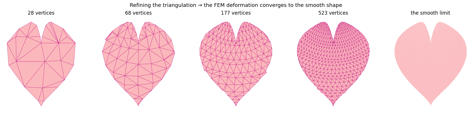
Apply this to every triangle at once. We sample the displacement only at the coarse vertices, then let each triangle interpolate its three corner vectors across its interior. That is a full finite-element deformation — no solver, no energy, just store-at-vertices + interpolate-inside.
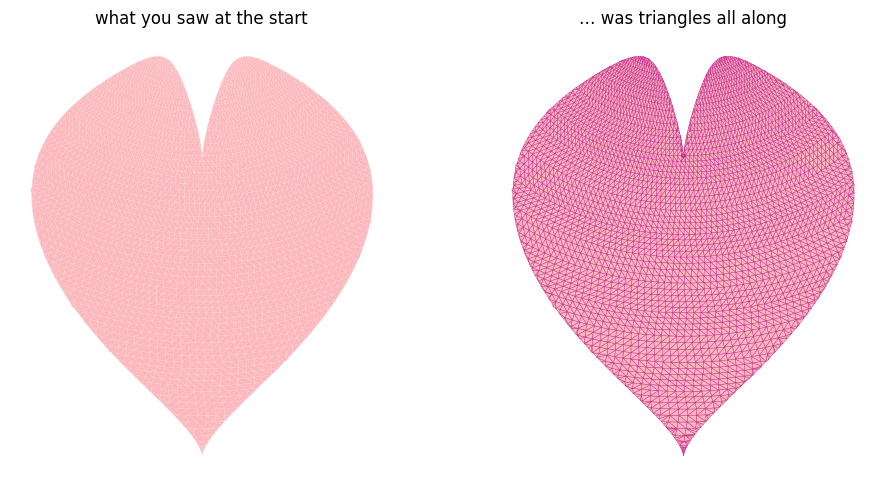
Now turn the triangle edges back on. The smooth deforming heart from the very first cell was a triangle mesh the entire time; we just never drew its edges. As we refine the mesh, the piecewise-linear approximation marches back toward the smooth limit you saw at the start.
# Refine the mesh from very coarse to fine; deform each by sampling u at its vertices.
levels = [(18, 0.5), (30, 0.26), (55, 0.14), (110, 0.075)]
meshes = [triangulate_heart(nb, sp) for (nb, sp) in levels]

fig, axes = plt.subplots(1, len(meshes) + 1, figsize=(3.4 * (len(meshes) + 1), 4))
for ax, (V, F) in zip(axes, meshes):
    show_shape(ax, deform(V), F, edges=True, title=f"{V.shape[0]} vertices")
show_shape(axes[-1], deform(X), T, edges=False, title="the smooth limit")
fig.suptitle("Refining the triangulation → the FEM deformation converges to the smooth shape",
             fontsize=13)
fig.tight_layout(); fig.savefig("media/00_convergence.png", dpi=130, bbox_inches="tight")
plt.show()
# The reveal: the same fine teaser heart, edges off vs edges on.
fig, axes = plt.subplots(1, 2, figsize=(10, 5))
show_shape(axes[0], deform(X), T, edges=False, title="what you saw at the start")
show_shape(axes[1], deform(X), T, edges=True, lw=0.3,
           title="… was triangles all along")
fig.tight_layout(); fig.savefig("media/00_reveal.png", dpi=130, bbox_inches="tight")
plt.show()
Takeaways#
The question “how does this shape deform?” is a request for a displacement field \(u(\bar x)\), i.e. one arrow per material point.
A computer can’t carry infinitely many arrows, so we discretize. The finite element method triangulates the shape, stores \(u\) only at the vertices, and reconstructs it everywhere else by barycentric interpolation with the linear basis functions \(\phi_i\): \(\,u(\bar x) = \sum_i \phi_i(\bar x)\, u_i.\)
Inside each triangle the deformation is just a linear blend of three corner vectors — the same blend we animated, applied everywhere at once.
Refine the mesh and the piecewise-linear field converges to the smooth one. The smooth teaser really was triangles the whole time.
With this foundation — how to represent a deformation on a computer — the rest of the tutorials build up the pipeline: measuring how stretched each element is (the deformation gradient, tutorial 1), turning that into an elastic energy, and minimizing it to actually find the deformation.
FEM is not the only way. Triangle/tet meshes are the classic choice, but they are one of many ways to discretize geometry and the fields living on it: Gaussian splats, RKPM and other meshless/particle methods, point clouds, signed distance fields, subdivision and spline patches, neural fields, and more. Each trades off smoothness, ease of meshing, adaptivity, and cost differently — and choosing the right discretization for a given geometry remains an active, open research problem.