19 · Compressed Vibration Modes: trading global modes for local ones#
Classical linear modal analysis (LMA) describes how an elastic body likes to vibrate. It diagonalizes the elastic energy against inertia — the generalized eigenproblem
with \(H\) the (linear-elasticity) stiffness and \(M\) the mass matrix. The eigenvectors \(u\) are the mode shapes. They are wonderful, but they share one stubborn property: every mode is global. A low-frequency mode of a beam is a sine wave that runs the entire length — touch one end and the whole shape responds. That is exactly the wrong basis if you want to edit, actuate, or simulate a body part by part.
Compressed modes fix this. Following “Compressed Vibration Modes of Elastic Bodies” (Brandt & Hildebrandt, 2017), we add an \(L_1\) penalty to the modal energy. Each mode now solves
The quadratic term still rewards smooth, low-energy shapes; the \(\lVert u\rVert_1\)
term rewards shapes that are exactly zero almost everywhere. The single knob
\(\lambda\) trades the two off. At \(\lambda = 0\) we recover ordinary LMA (global
modes); as \(\lambda\) grows, each mode shrinks its support and becomes a
local, sparse bump. simkit.eigs_iccm solves this problem — it
iteratively recasts each mode as a convex QP (splitting \(u = u_+ - u_-\) to
linearize the \(L_1\) term) and deflates against the modes already found.
In this tutorial we:
build a free-standing beam (pinned nowhere) and its \(H\), \(M\) operators,
compute the standard LMA modes and watch them oscillate — global,
crank \(\lambda\) up and watch the same modes localize,
quantify the sparsity directly.
All modes are shown by actuating them sinusoidally, \(x(t) = X + a\,\sin(2\pi t)\,u\) — no simulation, just the mode shape breathing in and out.
%matplotlib inline
import numpy as np
import scipy.sparse as sps
import matplotlib.pyplot as plt
from IPython.display import display

import simkit
import utils
from simkit.eigs_iccm import eigs_iccm
from simkit.energies.linear_elasticity import linear_elasticity_hessian

np.random.seed(0)
A free-standing beam#
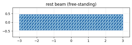
We mesh a long thin rectangle and pin nothing — the beam floats in space. Two matrices drive everything:
\(H\), the linear-elasticity stiffness (the Hessian of small-strain elastic energy). It is constant and positive semi-definite. Because the beam is unconstrained, \(H\) has a 3-dimensional null space: the two rigid translations and the in-plane rotation cost no energy.
\(M\), the mass matrix (lumped per-vertex mass, expanded to \(x\)/\(y\) DOFs).
These are exactly the ingredients of both LMA and the compressed-mode problem.
X, T = utils.triangulated_grid(40, 6, width=6.0, height=0.9)
n, dim = X.shape

mu = np.ones((T.shape[0], 1))                       # unit material; only the *shapes* matter
H  = linear_elasticity_hessian(X=X, T=T, mu=mu, lam=mu).tocsc()
M  = sps.kron(simkit.massmatrix(X, T), sps.identity(dim)).tocsc()

print(f"beam: {n} vertices, {T.shape[0]} triangles, {n*dim} DOFs")

fig, ax = plt.subplots(figsize=(7, 1.6))
utils.PolyMeshArtist(ax, X, T)
utils.setup_axes(ax, *utils.auto_limits([X]), title="rest beam (free-standing)")
plt.show()
beam: 240 vertices, 390 triangles, 480 DOFs
A tiny helper: actuate a mode sinusoidally#
Every mode is a column \(u \in \mathbb{R}^{n\cdot\text{dim}}\). To see it we
reshape it to a per-vertex displacement and sweep an amplitude through a full
sine period, \(x(t) = X + a\,\sin(2\pi t)\,u\). We rescale each mode so its largest
vertex displacement is the same on screen — otherwise mass-normalized modes
would have wildly different visual amplitudes. mode_panels packages one beam
per mode for utils.animate_meshes_grid, which plays them in sync.
def mode_disp(col):
    "(n*dim,) modal column -> (n, dim) per-vertex displacement."
    return col.reshape(n, dim)

def mode_panels(B, titles, n_frames=36, target=0.32):
    "One animation panel per column of B: the beam actuated sinusoidally."
    phases = np.sin(2 * np.pi * np.arange(n_frames) / n_frames)
    panels = []
    for j in range(B.shape[1]):
        d   = mode_disp(B[:, j])
        amp = target / (np.linalg.norm(d, axis=1).max() + 1e-12)   # equal screen amplitude
        panels.append({"states": [X + (amp * p) * d for p in phases],
                       "T": T, "title": titles[j]})
    return panels

def active_fraction(B, thresh=0.05):
    "Fraction of (vertex, mode) pairs that actually move (> 5% of that mode's peak)."
    mag = np.linalg.norm(B.reshape(n, dim, B.shape[1]), axis=1)
    return (mag > thresh * mag.max(axis=0)).mean()

mode_titles = [f"mode {i+1}" for i in range(5)]
Standard linear modal analysis — global modes#
simkit.linear_modal_analysis solves the plain generalized eigenproblem \(Hu =
\omega^2 M u\) for the lowest modes. The first three come back with eigenvalue
\(\approx 0\): those are the rigid-body modes (translate-\(x\), translate-\(y\),
rotate) that live in the null space of \(H\). We drop them and keep the first five
genuine deformation modes.
Watch the animation: every mode is a standing wave that occupies the whole beam. Mode \(k\) simply adds another half-wavelength. This is the global character we want to break.
E, Blma = simkit.linear_modal_analysis(X, T, k=8)
print("eigenvalues (omega^2):", np.round(E, 4), "  <- first 3 are rigid-body modes")

Blma = Blma[:, 3:8]                                 # first 5 deformation modes
fig, anim = utils.animate_meshes_grid(
    mode_panels(Blma, mode_titles), fps=18,
    suptitle="Linear modal analysis - every mode spans the whole beam")
print(f"active-vertex fraction: {active_fraction(Blma):.2f}  (nearly 1.0 - fully global)")
display(utils.show_video(fig, anim, "media/19_lma_modes.mp4", fps=18))
eigenvalues (omega^2): [-0.      0.      0.      0.0668  0.403   0.7292  1.2043  2.5513]   <- first 3 are rigid-body modes
active-vertex fraction: 1.00  (nearly 1.0 - fully global)
Turning on the sparsity knob \(\lambda\)#
Now we solve the compressed-mode problem with eigs_iccm, sweeping \(\lambda\).
Read the animations top to bottom:
\(\lambda = 0.5\) — light pressure. Modes still ripple over much of the beam, but the ends start going quiet.
\(\lambda = 2\) — each mode now lives in a region of the beam; the rest is frozen.
\(\lambda = 8\) — strong pressure. Modes collapse to compact, local bumps; only a small patch breathes while the remainder is rigid.
Same beam, same five modes — the only thing we changed is how much we charge for spreading out.
lambdas = [0.5, 2.0, 8.0]
Bs = {}
for l in lambdas:
    np.random.seed(0)                                # deterministic random init per sweep
    Bs[l] = eigs_iccm(H, l=l, k=5, M=M, max_iters=25)
    print(f"lambda = {l:>4}:  active-vertex fraction {active_fraction(Bs[l]):.2f}")
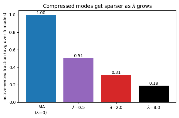
lambda = 0.5: active-vertex fraction 0.51
lambda = 2.0: active-vertex fraction 0.31
lambda = 8.0: active-vertex fraction 0.19
l = 0.5
fig, anim = utils.animate_meshes_grid(
    mode_panels(Bs[l], mode_titles), fps=18,
    suptitle=f"Compressed modes, lambda = {l}  (active fraction {active_fraction(Bs[l]):.2f})")
display(utils.show_video(fig, anim, f"media/19_iccm_l0.5.mp4", fps=18))
l = 2.0
fig, anim = utils.animate_meshes_grid(
    mode_panels(Bs[l], mode_titles), fps=18,
    suptitle=f"Compressed modes, lambda = {l}  (active fraction {active_fraction(Bs[l]):.2f})")
display(utils.show_video(fig, anim, f"media/19_iccm_l2.0.mp4", fps=18))
l = 8.0
fig, anim = utils.animate_meshes_grid(
    mode_panels(Bs[l], mode_titles), fps=18,
    suptitle=f"Compressed modes, lambda = {l}  (active fraction {active_fraction(Bs[l]):.2f})")
display(utils.show_video(fig, anim, f"media/19_iccm_l8.0.mp4", fps=18))
Seeing the support shrink directly#
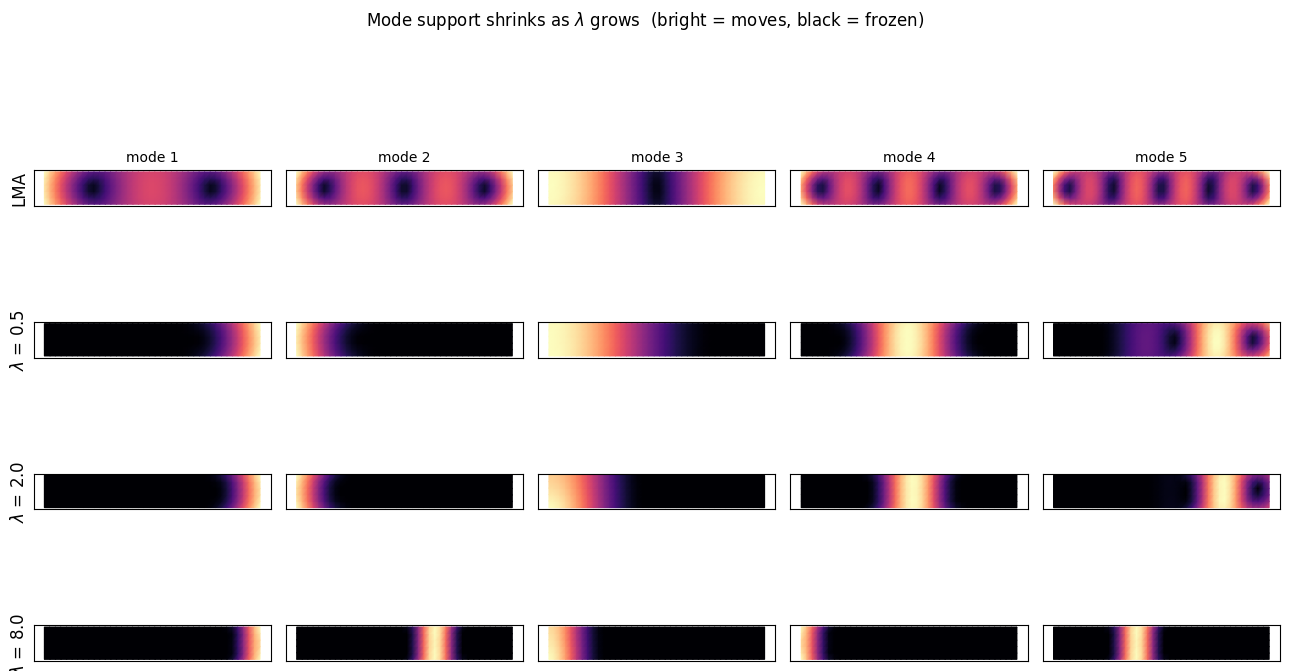
Animations show the motion; a heatmap of each mode’s per-vertex displacement magnitude on the rest beam shows the support at a glance. Bright = the vertex participates in that mode, black = it stays put. Top row is LMA; each row below raises \(\lambda\). The bright region contracts monotonically — the modes are literally becoming sparser.
def heatmap_row(axes, B):
    for ax, j in zip(axes, range(B.shape[1])):
        mag = np.linalg.norm(mode_disp(B[:, j]), axis=1)
        ax.tripcolor(X[:, 0], X[:, 1], T, mag / (mag.max() + 1e-12),
                     shading="gouraud", cmap="magma", vmin=0, vmax=1)
        ax.set_aspect("equal"); ax.set_xticks([]); ax.set_yticks([])

rows = [("LMA", Blma)] + [(f"$\\lambda$ = {l}", Bs[l]) for l in lambdas]
fig, axes = plt.subplots(len(rows), 5, figsize=(13, 1.9 * len(rows)))
for r, (name, B) in enumerate(rows):
    heatmap_row(axes[r], B)
    axes[r][0].set_ylabel(name, fontsize=12)
    if r == 0:
        for j in range(5):
            axes[0][j].set_title(f"mode {j+1}", fontsize=10)
fig.suptitle("Mode support shrinks as $\\lambda$ grows  (bright = moves, black = frozen)", y=1.01)
fig.tight_layout()
fig.savefig("media/19_heatmaps.png", dpi=110, bbox_inches="tight")
plt.show()
Quantifying sparsity#
The “active-vertex fraction” — the share of vertices whose displacement exceeds 5% of a mode’s peak, averaged over the five modes — falls off steeply with \(\lambda\). LMA modes touch essentially every vertex; by \(\lambda = 8\) each mode lives on a small fraction of the beam.
xs = ["LMA\n($\\lambda$=0)"] + [f"$\\lambda$={l}" for l in lambdas]
ys = [active_fraction(Blma)] + [active_fraction(Bs[l]) for l in lambdas]

fig, ax = plt.subplots(figsize=(6, 4))
ax.bar(xs, ys, color=["#1f77b4", "#9467bd", "#d62728", "#000000"])
for i, v in enumerate(ys):
    ax.text(i, v + 0.01, f"{v:.2f}", ha="center", fontsize=10)
ax.set_ylim(0, 1.05); ax.set_ylabel("active-vertex fraction (avg over 5 modes)")
ax.set_title("Compressed modes get sparser as $\\lambda$ grows")
fig.tight_layout(); fig.savefig("media/19_sparsity.png", dpi=110)
plt.show()
Takeaways#
LMA modes are global. They diagonalize \(H\) against \(M\), and the low-frequency shapes inevitably span the whole body. Great for spectral analysis, awkward for local editing.
An \(L_1\) penalty buys locality. Minimizing \(\tfrac12 u^\top H u + \lambda \lVert u\rVert_1\) (mass-normalized, deflated) keeps the modes smooth where they live but forces them to zero everywhere else.
One knob. \(\lambda\) slides continuously from global LMA (\(\lambda\to 0\)) to tightly localized bumps (large \(\lambda\)) — we watched both the motion and the support change with nothing else touched.
simkit.eigs_iccmcomputes these compressed modes for any \((H, M)\) pair, so the same recipe applies to any mesh, not just this beam.
Localized modes are a natural basis for part-based deformation, sparse control / actuation, and domain-decomposed reduced simulation — places where a global modal basis would couple everything to everything.