18 · Rotation–Strain Coordinates: Rescuing a Linear Mode#
A linear mode is the cheapest way to make a shape move: precompute a displacement field \(\phi\) once, then actuate it as \(x(a)=X+a\,\phi\). One scalar \(a\) drives the whole deformation. It is linear in \(a\) — and that is exactly the problem.
Real deformation rotates. When a cantilever bends, its tip swings along an arc; each little element turns. But a linear mode can only translate every vertex along a fixed straight line \(\phi_i\). For small \(a\) a straight line is a fine approximation to the arc. For large \(a\) it is not: the tip shoots off tangent to the arc instead of following it, the beam stretches, elements shear, and — pushed far enough — invert (negative area, turned inside-out). These are linearization artifacts: spurious strain that a true rotation would never produce.
Rotation–strain (RS) coordinates fix this — not by deleting strain, but by upgrading the rotation. Split each element’s displacement gradient \(\nabla u\) into its two additive parts: an antisymmetric piece (the rotation generator — how much the element is turning) and a symmetric piece (the genuine strain — how much it is actually stretching). A linear mode reads the turn back only to first order, \(F=I+\nabla u\), and \(I+(\text{a small rotation})\) is a lousy rotation: it inflates area. RS coordinates instead exponentiate the rotation generator into a true finite rotation \(R\) (Rodrigues’ formula), reapply it to the genuine stretch \(S=I+\mathrm{sym}(\nabla u)\), set the per-element target to \(R\,S-I\), and refit a single displacement field whose Jacobian reproduces it. The spurious area inflation from the linearized turn disappears; the real stretch is kept exactly.
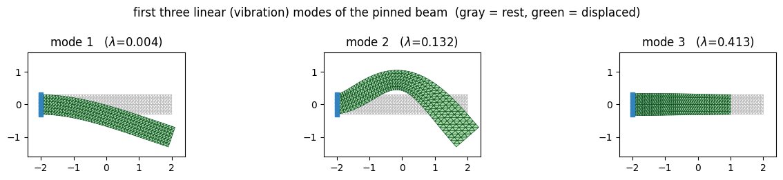
We will (1) pin a beam and pull out its first three linear modes — two
bending modes that are mostly rotation, and one longitudinal mode that is
genuine stretch; (2) actuate a bending mode sinusoidally with a
swelling-then-shrinking amplitude and watch the shearing / inflation / inversion
artifacts grow; (3) reinterpret that same actuated field through
rotation_strain_coordinates and watch the spurious inflation vanish while the
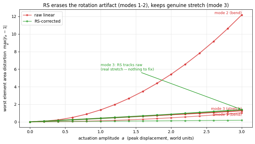
bend follows a true arc; and (4) chart area distortion vs. amplitude across all
three modes to show the punchline — RS erases the rotation artifact
(modes 1–2) but faithfully preserves genuine strain (mode 3). It fixes
what’s fake and keeps what’s real.
%matplotlib inline
import numpy as np
import matplotlib.pyplot as plt
from matplotlib.animation import FuncAnimation
from matplotlib.collections import PolyCollection
from matplotlib.colors import TwoSlopeNorm

import simkit
import utils

LIN_C  = "#d62728"   # linear mode (raw) -- has artifacts
RS_C   = "#2ca02c"   # rotation-strain corrected
REST_C = "#bdbdbd"   # ghost of the rest beam
PIN_C  = "#3182bd"   # pinned wall


def signed_areas(V, T):
    """Per-triangle signed area; negative means the element has flipped."""
    return 0.5 * ((V[T[:, 1], 0] - V[T[:, 0], 0]) * (V[T[:, 2], 1] - V[T[:, 0], 1])
                - (V[T[:, 1], 1] - V[T[:, 0], 1]) * (V[T[:, 2], 0] - V[T[:, 0], 0]))


class AreaMeshArtist:
    """A triangle mesh colored per-element by area ratio (deformed / rest).

    Red = inflated, white = volume-preserving (ratio 1, what a rigid rotation
    gives), blue = compressed/inverted. ``update`` moves it to a new state."""

    def __init__(self, ax, U, T, ratio, vmax=2.0):
        self.T = np.asarray(T)
        self.norm = TwoSlopeNorm(vmin=0.0, vcenter=1.0, vmax=vmax)
        self.coll = PolyCollection([U[f] for f in self.T], array=np.asarray(ratio),
                                   cmap="RdBu_r", norm=self.norm,
                                   edgecolors="0.25", linewidths=0.3, zorder=2)
        ax.add_collection(self.coll)

    def update(self, U, ratio):
        self.coll.set_verts([U[f] for f in self.T])
        self.coll.set_array(np.asarray(ratio))
A cantilever beam, pinned on the left#
A right-triangulated rectangular beam, clamped along its left edge. Pinning is what makes the modes interesting: the free end is what swings through a large angle, so it is where the linear approximation breaks first.
nx, ny = 48, 7
X, T = utils.triangulated_grid(nx, ny, width=4.0, height=0.6)
n, dim = X.shape
pin = np.where(X[:, 0] <= X[:, 0].min() + 1e-6)[0]   # clamp the whole left edge
print(f"beam: {n} vertices, {T.shape[0]} triangles, {n*dim} DOFs")
print(f"pinned (left wall): {pin.size} vertices")
beam: 336 vertices, 564 triangles, 672 DOFs
pinned (left wall): 7 vertices
The first three linear modes#
simkit.linear_modal_analysis solves the generalized eigenproblem
\(K\,\phi=\lambda\,M\,\phi\) for the ARAP stiffness \(K\) and mass \(M\), with the
pinned DOFs eliminated, and returns the lowest modes sorted by eigenvalue
\(\lambda\) (squared frequency). The first mode is the softest — the
fundamental bend; the second is the next bend (an S-shape with one interior
node); the third here is a longitudinal stretch mode.
They are all fixed displacement fields, but they differ in what their Jacobian encodes. The two bending modes are dominated by the antisymmetric (rotation) part of \(\nabla u\) — each element mostly turns — while the stretch mode is dominated by the symmetric (strain) part — each element mostly stretches. That distinction is exactly what RS coordinates key off: it fixes the rotation-dominated modes and leaves the stretch one alone.
Each \(\phi\) comes out mass-normalized, so we rescale every mode to unit peak displacement — then an actuation amplitude \(a\) reads directly as the distance, in world units, that the most-displaced vertex moves.
k = 3
E, B = simkit.linear_modal_analysis(X, T, k, bI=pin)
modes = [B[:, i].reshape(n, dim) for i in range(k)]
modes = [m / np.abs(m).max() for m in modes]          # unit peak displacement
print("eigenvalues (squared frequency):", np.round(E[:k], 4))

fig, axes = plt.subplots(1, k, figsize=(13, 2.6))
amp_show = 1.0
for i, (ax, m) in enumerate(zip(axes, modes)):
    utils.setup_axes(ax, (-2.4, 2.4), (-1.6, 1.6),
                     title=f"mode {i+1}   ($\\lambda$={E[i]:.3f})", grid=False)
    ax.add_collection(PolyCollection([X[f] for f in T], facecolors="none",
                                     edgecolors=REST_C, linewidths=0.6, zorder=1))
    Um = X + amp_show * m
    ax.add_collection(PolyCollection([Um[f] for f in T], facecolors="#a1d99b",
                                     edgecolors="#00441b", linewidths=0.5,
                                     alpha=0.9, zorder=2))
    ax.scatter(X[pin, 0], X[pin, 1], s=22, color=PIN_C, marker="s", zorder=4)
fig.suptitle("first three linear (vibration) modes of the pinned beam  "
             "(gray = rest, green = displaced)")
fig.tight_layout(); fig.savefig("media/18_modes.png", dpi=130, bbox_inches="tight")
plt.show()
eigenvalues (squared frequency): [0.0041 0.132 0.4134]
Actuate the first mode — sinusoidally, swelling then fading#
We drive the fundamental bending mode with
one full sine period: the tip swings up to \(+A_{\max}\), back through rest, down to \(-A_{\max}\), and home again — the actuation magnitude rising, then falling, then rising, then falling. We push \(A_{\max}\) deliberately large so the artifact is unmistakable.
Each frame is colored by area ratio (deformed element area / rest area). A rigid rotation preserves area, so a faithful bend should stay white (ratio 1) everywhere. Watch instead: as the tip swings out, the elements near it flush red — the straight-line mode stretches the beam because the tip leaves along the tangent instead of riding the arc. The trace on the right tracks the worst element; it spikes at every swing and only returns to 1 as the beam passes back through rest.
A_max = 3.0
mode = modes[0]
n_frames = 61
tt = np.linspace(0.0, 1.0, n_frames)
a_t = A_max * np.sin(2.0 * np.pi * tt)               # one full sine period
A0 = signed_areas(X, T)

states_lin, ratio_lin, peak_lin = [], [], []
for a in a_t:
    U = X + a * mode
    r = signed_areas(U, T) / A0
    states_lin.append(U)
    ratio_lin.append(r)
    peak_lin.append(r.max())
peak_lin = np.array(peak_lin)
print(f"raw linear mode at A_max={A_max}:  peak area ratio {peak_lin.max():.2f}x"
      f"   min element area ratio {min(r.min() for r in ratio_lin):+.2f}"
      f"  (negative => inverted elements)")

fig, (axL, axR) = plt.subplots(1, 2, figsize=(13, 4.4),
                               gridspec_kw={"width_ratios": [1.35, 1]})
utils.setup_axes(axL, (-2.4, 4.4), (-3.2, 3.2),
                 title="linear actuation $x=X+a\\,\\phi$  (color = area ratio)", grid=False)
art = AreaMeshArtist(axL, states_lin[0], T, ratio_lin[0], vmax=2.0)
axL.scatter(X[pin, 0], X[pin, 1], s=26, color=PIN_C, marker="s", zorder=4)
fig.colorbar(art.coll, ax=axL, fraction=0.046, pad=0.02,
             label="area ratio  (1 = rigid)")
trace = utils.TracePlot(axR, tt, {"raw linear mode": peak_lin},
                        colors={"raw linear mode": LIN_C},
                        xlabel="actuation phase  $t$", ylabel="peak area ratio  (max over elements)",
                        title="straight-line actuation inflates area")
axR.axhline(1.0, color="0.5", ls="--", lw=1.2, zorder=1)

def update(i):
    art.update(states_lin[i], ratio_lin[i])
    trace.update(i)
    return ()

anim = FuncAnimation(fig, update, frames=n_frames, interval=1000/20, blit=False)
fig.tight_layout()
update(int(np.argmax(peak_lin)))   # freeze on a peak-swing frame for the saved still
fig.savefig("media/18_linear_artifacts.png", dpi=130, bbox_inches="tight")
utils.show_video(fig, anim, "media/18_linear_artifacts.mp4", fps=20)
raw linear mode at A_max=3.0: peak area ratio 2.03x min element area ratio +0.82 (negative => inverted elements)
Reinterpret the actuation in rotation–strain coordinates#
The red flush is not real strain — it is the linearized rotation faking it. A true rotation preserves area; the first-order stand-in \(I+\nabla u\) does not. Here is how RS coordinates separate the fake from the real, element by element:
From the linear field \(u=a\,\phi\) form the deformation gradient \(F=I+\nabla u\) on every element (
deformation_jacobiansupplies \(\nabla u\)), and split \(\nabla u\) into its two additive halves: $\( \nabla u \;=\; \underbrace{\mathrm{skew}(\nabla u)}_{W\ \text{(rotation generator)}} \;+\; \underbrace{\mathrm{sym}(\nabla u)}_{\text{strain}}. \)$Upgrade the rotation. \(W\) is only an infinitesimal rotation — the axis–angle the linear field encodes. Exponentiate it into a genuine finite rotation \(R=\exp(W)\). In 2D, \(W=\big[\begin{smallmatrix}0&-w\\ w&0\end{smallmatrix}\big]\) and \(R\) is rotation by the angle \(w\); in 3D this is Rodrigues’ formula. Unlike \(I+W\), the matrix \(R\) is a true rotation — \(\det R=1\), area preserved exactly.
Keep the real strain. Form \(S=I+\mathrm{sym}(\nabla u)\), set the per-element target \(Y=R\,S-I\) — rotation exponentiated, strain untouched — and solve one small least-squares fit for the displacement \(u_{\text{rs}}\) whose Jacobian best matches \(Y\) everywhere (a pinned Poisson-type solve, prefactored once in
RSPrecompute).
So RS coordinates read the linear mode’s rotation content and rebuild it as an
actual rotation, while passing genuine stretch through unchanged.
simkit.rotation_strain_coordinates returns that \(u_{\text{rs}}\) (and a reusable
precompute). We run it on every frame of the same actuation and compare side
by side. Because this bending mode is rotation-dominated, almost all of its
distortion was the linearization artifact — so RS should knock it right
down.
states_rs, ratio_rs, peak_rs = [], [], []
pre = None                                            # RSPrecompute: build once, reuse
for a in a_t:
    u = (a * mode).reshape(-1)
    u_rs, pre = simkit.rotation_strain_coordinates(X, T, u, pinned=pin, pre=pre)
    U = X + u_rs
    r = signed_areas(U, T) / A0
    states_rs.append(U)
    ratio_rs.append(r)
    peak_rs.append(r.max())
peak_rs = np.array(peak_rs)
print(f"raw linear : peak area ratio {peak_lin.max():.2f}x")
print(f"RS-corrected: peak area ratio {peak_rs.max():.2f}x   "
      f"(linearized-rotation inflation removed; small genuine bending strain remains)")

fig, (axA, axB, axR) = plt.subplots(1, 3, figsize=(15, 4.4),
                                    gridspec_kw={"width_ratios": [1, 1, 1.05]})
utils.setup_axes(axA, (-2.4, 4.4), (-3.2, 3.2), title="raw linear mode", grid=False)
utils.setup_axes(axB, (-2.4, 4.4), (-3.2, 3.2), title="rotation-strain coordinates", grid=False)
aA = AreaMeshArtist(axA, states_lin[0], T, ratio_lin[0], vmax=2.0)
aB = AreaMeshArtist(axB, states_rs[0],  T, ratio_rs[0],  vmax=2.0)
for ax in (axA, axB):
    ax.scatter(X[pin, 0], X[pin, 1], s=26, color=PIN_C, marker="s", zorder=4)
fig.colorbar(aB.coll, ax=axB, fraction=0.046, pad=0.02, label="area ratio  (1 = rigid)")
trace = utils.TracePlot(axR, tt, {"raw linear": peak_lin, "RS-corrected": peak_rs},
                        colors={"raw linear": LIN_C, "RS-corrected": RS_C},
                        xlabel="actuation phase  $t$", ylabel="peak area ratio",
                        title="RS removes the spurious area inflation")
axR.axhline(1.0, color="0.5", ls="--", lw=1.2, zorder=1)

def update(i):
    aA.update(states_lin[i], ratio_lin[i])
    aB.update(states_rs[i],  ratio_rs[i])
    trace.update(i)
    return ()

anim = FuncAnimation(fig, update, frames=n_frames, interval=1000/20, blit=False)
fig.tight_layout()
update(int(np.argmax(peak_lin)))   # freeze on a peak-swing frame for the saved still
fig.savefig("media/18_rs_vs_linear.png", dpi=130, bbox_inches="tight")
utils.show_video(fig, anim, "media/18_rs_vs_linear.mp4", fps=20)
raw linear : peak area ratio 2.03x
RS-corrected: peak area ratio 1.18x   (linearized-rotation inflation removed; small genuine bending strain remains)
How bad does it get? Distortion vs. amplitude#
The animation is one amplitude sweep of one mode; this is the whole story in one chart. For a range of actuation amplitudes \(a\) we measure the worst element area distortion \(\max_e |r_e - 1|\) for each of the three modes, raw vs. RS-corrected.
The two bending modes (1, 2) are rotation-dominated. Their raw distortion climbs without bound — roughly linearly with \(a\), fastest for the higher mode (more curvature, more rotation packed into each element, even flipping them) — but that distortion is fake, a linearization-of-rotation artifact, and RS collapses it toward flat by exponentiating the turn.
The stretch mode (3) is the control. Its distortion is genuine strain, not a rotation artifact, so there is nothing for RS to remove: the RS curve tracks the raw curve almost exactly. That is the whole point of doing this correctly — RS erases spurious rotation-stretch and preserves real stretch, rather than bulldozing both to zero. (The old “rotation-only” variant would have wrongly flattened mode 3 too.)
amps = np.linspace(0.0, 3.0, 16)
fig, ax = plt.subplots(figsize=(8.8, 5.0))
pres = [None, None, None]
for i, m in enumerate(modes):
    d_lin, d_rs = [], []
    for a in amps:
        U = X + a * m
        d_lin.append(np.abs(signed_areas(U, T) / A0 - 1.0).max())
        u_rs, pres[i] = simkit.rotation_strain_coordinates(
            X, T, (a * m).reshape(-1), pinned=pin, pre=pres[i])
        d_rs.append(np.abs(signed_areas(X + u_rs, T) / A0 - 1.0).max())
    ax.plot(amps, d_lin, "-o", color=LIN_C, lw=2, ms=4, alpha=0.55 + 0.15*i,
            label="raw linear" if i == 0 else None)
    ax.plot(amps, d_rs, "-o", color=RS_C, lw=2, ms=4, alpha=0.55 + 0.15*i,
            label="RS-corrected" if i == 0 else None)
    kind = "stretch" if i == 2 else "bend"
    # mode 1's raw endpoint sits just under mode 3's, so drop its label below the
    # point (va="top") to keep the two from colliding at the right edge.
    ax.annotate(f"mode {i+1} ({kind})", (amps[-1], d_lin[-1]), color=LIN_C,
                fontsize=9, ha="right", va="top" if i == 0 else "bottom")
# Mode 3 is genuine stretch: RS preserves it, so its green (RS) curve lands right
# on top of the red (raw) one -- nothing to remove, unlike the bending modes.
ax.annotate("mode 3: RS tracks raw\n(real stretch -- nothing to fix)",
            xy=(amps[-1], d_rs[-1]), xytext=(1.0, 6.2), color=RS_C, fontsize=9,
            ha="left", va="center",
            arrowprops=dict(arrowstyle="->", color=RS_C, lw=1.3))
ax.set_xlabel("actuation amplitude  $a$  (peak displacement, world units)")
ax.set_ylabel("worst element area distortion  $\\max_e |r_e-1|$")
ax.set_title("RS erases the rotation artifact (modes 1-2), keeps genuine stretch (mode 3)")
ax.grid(True, color="0.9"); ax.legend(loc="upper left")
fig.tight_layout(); fig.savefig("media/18_distortion_vs_amp.png", dpi=130, bbox_inches="tight")
plt.show()
Takeaways#
A linear mode \(x=X+a\,\phi\) moves every vertex along a fixed straight line. Cheap and great for small \(a\), but rotation is nonlinear in position, so at large \(a\) the straight line departs the true arc: the shape stretches, shears, and inverts. These linearization artifacts show up directly as area ratios far from 1.
Rotation–strain coordinates split the linear field’s Jacobian additively into an antisymmetric rotation generator \(W=\mathrm{skew}(\nabla u)\) and a symmetric strain \(\mathrm{sym}(\nabla u)\). They exponentiate the rotation generator into a true finite rotation \(R=\exp(W)\) — it had been read back only to first order, \(I+W\), which inflates area — keep the genuine stretch \(S=I+\mathrm{sym}(\nabla u)\), and refit a displacement whose Jacobian is \(R\,S-I\). The turn is upgraded; the stretch is preserved.
The payoff cuts both ways. The same one-scalar actuation now bends the beam along a true arc with the spurious area inflation gone (modes 1–2) — and it does this without erasing genuine deformation: a real stretch mode keeps its stretch (mode 3’s RS curve tracks the raw mode). RS removes only the fake rotation-stretch; it does not flatten real strain.
Use it whenever a cheap linear subspace has to undergo large rotation — actuated characters, cables, tentacles, modal animation — to get rotation-aware motion at linear-mode cost. It is the same lesson as the skinning-eigenmodes tutorial (17), reached from the other direction: there we built a rotation-capable basis; here we repair a rotation-blind one after the fact.
RS coordinates turn a rotation-blind linear mode into a rotation-aware one by exponentiating the turn its Jacobian already encodes — and keeping the genuine strain intact — the same neo-Hookean-era kinematics (tutorials 1–3), now in service of cheap actuation.