24 · Subspace Mixed FEM (MFEM)#
We simulate an elastic 2D beam dropping under gravity, pinned at its left edge, two ways:
Full-space FEM — the classic recipe. One Newton solve per timestep on the elastic + inertial + pin energy, written as a function of the deformed positions.
Subspace Mixed FEM (MFEM) — the method of Trusty et al., Subspace Mixed FEM. We solve in a small skinning-eigenmode subspace and introduce an auxiliary stretch variable so the elastic energy stays element-local and cheap, even though the subspace basis is dense.
Each method is packaged as a small simulator object: a FEMBeam baseline that
drives newton_solver on one energy, and an MFEMBeam that drives sqp_mfem
on the mixed energy and its Hessian/gradient blocks.
Why a subspace, and why “mixed”?#
A reduced model writes every vertex position as
where \(B\) is a tall dense basis (here, skinning eigenmodes) and \(\mathbf{u}\) is a handful of reduced weights. Stepping then solves for \(\mathbf{u}\) only, which is great — until you evaluate the elastic energy. The elastic Hessian in the subspace is \(B^\top H B\): dense, and expensive to assemble because \(H\) couples the deformation gradient \(F = \nabla(B\mathbf{u})\) across all elements.
Mixed FEM breaks that coupling. Introduce a per-element auxiliary stretch variable \(\mathbf{a}\) (the symmetric part of \(F\), one small vector per cubature element) and demand that it agree with the actual deformation:
Now the elastic energy is a function of \(\mathbf{a}\) alone — fully element-local, so its Hessian \(H_z\) is block-diagonal and trivial to build. The only thing tying \(\mathbf{a}\) back to the dense subspace is the constraint, whose Jacobian \(G_u\) is cheap. We minimize the Lagrangian
%matplotlib inline
import numpy as np
import scipy as sp
import matplotlib.pyplot as plt
from matplotlib import animation

import simkit as sk
from simkit.solvers import sqp_mfem, newton_solver
from simkit.energies import (
    elastic_energy_S, elastic_gradient_S, elastic_hessian_S,        # element-local (stretch) energy
    elastic_energy_z, elastic_gradient_z, elastic_hessian_z, ElasticEnergyZPrecomp,  # FEM (subspace) energy
    quadratic_energy, quadratic_gradient, quadratic_hessian,        # pin + gravity
    kinetic_energy_be, kinetic_gradient_be, kinetic_hessian_be,     # backward-Euler inertia
)
import utils

# sparse @ on some scipy/numpy combos emits spurious 'divide by zero in matmul'
# warnings; the arithmetic is exact. Silence them for a clean notebook.
np.seterr(all="ignore")
{'divide': 'warn', 'over': 'warn', 'under': 'ignore', 'invalid': 'warn'}
The mesh, subspace, and cubature#
A long thin beam. We build:
B— a skinning-eigenmode subspace (sk.skinning_eigenmodes).x = B @ u + q, withqthe rest geometry, sou = 0is the rest pose.cI, cW— spectral cubature points and weights (sk.spectral_cubature): a sparse subset of elements (with weights) at which we evaluate the elastic energy, instead of all of them.
X, T = utils.triangulated_grid(nx=40, ny=8, width=3.0, height=0.5)
n, dim = X.shape
q = X.reshape(-1, 1)                       # rest geometry offset:  x = B u + q

ym, pr, rho, h = 1e5, 0.45, 1e3, 1e1       # Young's modulus, Poisson, density, timestep
material = "macklin-mueller-neo-hookean"

# skinning-eigenmode subspace + spectral cubature
m, k = 10, 400
mu_tet = np.full((T.shape[0], 1), float(ym))
W, E, B = sk.skinning_eigenmodes(X, T, m, mu=mu_tet)
cI, cW, _ = sk.spectral_cubature(X, T, W, k, return_labels=True)
print(f"{n} vertices, {T.shape[0]} triangles, {n*dim} full DOFs")
print(f"subspace dim = {B.shape[1]},  cubature points = {cI.shape[0]}")
320 vertices, 546 triangles, 640 full DOFs
subspace dim = 60,  cubature points = 400
The MFEM simulator and its blocks#
We solve for the stacked state \(\mathbf{p} = [\mathbf{u};\,\mathbf{a};\,\boldsymbol{\lambda}]\)
— subspace positions, per-cubature stretch auxiliaries, and the Lagrange
multipliers \(\boldsymbol{\lambda}\) of the constraint \(\mathbf{c}=S(F(\mathbf u))-\mathbf a=0\).
sqp_mfem minimises the augmented-Lagrangian merit
updating the primal \([\mathbf u;\mathbf a]\) and overwriting \(\boldsymbol\lambda\) with the freshly computed multiplier each iteration. The simulator exposes:
energy(p)— the scalar merit, written as a sum of named terms (E_elastic,E_kinetic,E_quadpin+gravity,E_lag,E_aug).grad_blocks(p) -> [f_u, f_z, f_ll]— the objective + penalty gradient w.r.t. positions and stretch (the multiplier coupling \(+G_u\boldsymbol\lambda\), \(-W\boldsymbol\lambda\) is added by the solver), and the weighted constraint residual \(f_{\lambda}=W\mathbf c\).hess_blocks(p) -> [H_u, H_z, G_u, G_z, G_zi]— position Hessian (inertia + pin \(+\,\rho_{\text{aug}}G_uW^{-1}G_u^\top\), a Gauss-Newton penalty term), block-diagonal stretch Hessian \(H_z+\rho_{\text{aug}}W\), constraint Jacobian \(G_u=\frac{\partial S}{\partial u}^\top W\), \(G_z=-W\), and \(G_z^{-1}\).
rho_aug is an optional augmentation that can stabilise the line search; we study
its effect on convergence below.
class MFEMBeam:
    """Subspace mixed FEM: drives `sqp_mfem` on the stacked state [u; a; ll]."""

    def __init__(self, GJB, GJq, Ci, kin_pre, BQB, Bb, w, Wd, Wi, h, mu, lam, vol,
                 material, nz, na, dim, B, X, T, q, rho_aug=0.0):
        self.GJB, self.GJq, self.Ci = GJB, GJq, Ci
        self.kin_pre, self.BQB, self.Bb = kin_pre, BQB, Bb
        self.w, self.Wd, self.Wi = w, Wd, Wi
        self.h, self.mu, self.lam, self.vol = h, mu, lam, vol
        self.material, self.nz, self.na, self.dim = material, nz, na, dim
        self.B, self.X, self.T, self.q = B, X, T, q
        self.rho_aug = rho_aug

    def split(self, p):
        nz, na = self.nz, self.na
        return p[:nz], p[nz:nz+na], p[nz+na:]       # u (positions), a (stretch), ll (multiplier)

    def energy(self, p, z_curr, z_prev, ra):
        u, a, ll = self.split(p)
        A = a.reshape(-1, self.dim*(self.dim+1)//2)
        F = (self.GJB @ u + self.GJq).reshape(-1, self.dim, self.dim)
        c  = self.Ci @ sk.stretch(F) - a                  # stretch constraint residual
        wc = self.w * c                                   # = W c
        E_elastic = elastic_energy_S(A, self.mu, self.lam, self.vol, self.material)
        E_kinetic = kinetic_energy_be(u, z_curr, z_prev, self.kin_pre, self.h)
        E_quad    = quadratic_energy(u, self.BQB, self.Bb)        # pin + gravity
        E_lag     = float((ll.T @ wc)[0, 0])                             # ll^T W c
        E_aug     = 0.5 * ra * float((c.T @ wc)[0, 0])                   # 0.5 rho c^T W c
        return E_elastic + E_kinetic + E_quad + E_lag + E_aug

    def grad_blocks(self, p, z_curr, z_prev, ra):
        u, a, ll = self.split(p)
        A = a.reshape(-1, self.dim*(self.dim+1)//2)
        F = (self.GJB @ u + self.GJq).reshape(-1, self.dim, self.dim)
        wc   = self.w * (self.Ci @ sk.stretch(F) - a)
        dsdz = sk.stretch_gradient_dz(u, self.GJB, Ci=self.Ci, dim=self.dim, GJq=self.GJq)
        # d/du of 0.5 rho c^T W c is rho * dsdz @ (W c) = rho * dsdz @ wc
        # (NOT G_u @ wc = dsdz @ W @ wc, which double-weights the off-diagonals by W).
        g_kinetic = kinetic_gradient_be(u, z_curr, z_prev, self.kin_pre, self.h)
        g_quad    = quadratic_gradient(u, self.BQB, self.Bb)
        g_aug     = ra * (dsdz @ wc)
        f_u  = g_kinetic + g_quad + g_aug
        f_z  = elastic_gradient_S(A, self.mu, self.lam, self.vol, self.material).reshape(-1, 1) - ra * wc   # dc/da = -I
        f_ll = wc                                         # constraint residual (W c)
        return [f_u, f_z, f_ll]

    def hess_blocks(self, p, z_curr, z_prev, ra):
        u, a, ll = self.split(p)
        A = a.reshape(-1, self.dim*(self.dim+1)//2)
        dsdz = sk.stretch_gradient_dz(u, self.GJB, Ci=self.Ci, dim=self.dim, GJq=self.GJq)
        G_u  = dsdz @ self.Wd
        H_inertia = kinetic_hessian_be(self.kin_pre, self.h)
        H_pin     = quadratic_hessian(self.BQB)
        H_pen     = ra * (G_u @ self.Wi @ G_u.T)
        H_u  = H_inertia + H_pin + H_pen
        H_z  = sp.sparse.block_diag([hh for hh in elastic_hessian_S(A, self.mu, self.lam, self.vol, self.material)]) + ra * self.Wd
        G_z  = -self.Wd
        G_zi = sp.sparse.diags(1.0 / G_z.diagonal())
        return [H_u, H_z, G_u, G_z, G_zi]

    def rest_state(self):
        u = sk.project_into_subspace(self.X.reshape(-1,1) - self.q, self.B,
                M=sp.sparse.kron(sk.massmatrix(self.X, self.T), sp.sparse.identity(self.dim)))
        ncub = self.na // (self.dim*(self.dim+1)//2)               # number of cubature points
        a = np.ones((ncub, self.dim*(self.dim+1)//2))
        a[:, self.dim:] = 0.0                                       # identity stretch
        ll = np.zeros((self.na, 1))                                 # zero multiplier
        return u, a.reshape(-1, 1), ll

    def step(self, z_curr, z_prev, a, ll):
        p = np.vstack([z_curr, a, ll])
        p = sqp_mfem(p,
                     lambda pp: self.energy(pp, z_curr, z_prev, self.rho_aug),
                     lambda pp: self.hess_blocks(pp, z_curr, z_prev, self.rho_aug),
                     lambda pp: self.grad_blocks(pp, z_curr, z_prev, self.rho_aug),
                     tolerance=1e-6, max_iter=30, do_line_search=True)
        return self.split(p)

mfem = MFEMBeam(GJB, GJq, Ci, kin_pre, BQB, Bb, w, Wd, Wi, h, mu, lam, vol,
                material, nz, na, dim, B, X, T, q, rho_aug=rho_aug)
Verifying the blocks (finite differences)#
Before trusting the solve, check the blocks against central finite differences of the scalar merit \(E(\mathbf p)\):
grad_blocksreproduce \(\nabla E\) once the multiplier coupling the solver adds (\(+G_u\boldsymbol\lambda\), \(+G_z\boldsymbol\lambda\)) is included — for \(\rho_{\text{aug}}=0\) and \(\rho_{\text{aug}}>0\).\(H_z=\partial^2E/\partial\mathbf a^2\) exactly.
\(H_u\) is a Gauss-Newton Hessian: it matches \(\partial^2E/\partial\mathbf u^2\) exactly at \(\boldsymbol\lambda=0,\rho_{\text{aug}}=0\) and stays SPD (what the condensed solve needs) for all \(\rho_{\text{aug}}\ge 0\).
The same checks live in tests/test_mfem_blocks.py.
from simkit.gradient_cfd import gradient_cfd
def _dense(M):
    return np.asarray(M.todense()) if sp.sparse.issparse(M) else np.asarray(M)
def _tag(r, tol=1e-4):
    return "PASS" if r < tol else "FAIL"

_rng = np.random.default_rng(0)
_u, _a, _ll = mfem.rest_state()
_u  = _u + 0.05 * _rng.standard_normal(_u.shape)
_a  = _a + 0.05 * _rng.standard_normal(_a.shape)
_ll = 0.05 * _rng.standard_normal(_ll.shape)
_zc = _zp = mfem.rest_state()[0]

def _verify(ra):
    p = np.vstack([_u, _a, _ll])
    f_u, f_z, f_ll = mfem.grad_blocks(p, _zc, _zp, ra)
    H_u, H_z, G_u, G_z, G_zi = mfem.hess_blocks(p, _zc, _zp, ra)
    # full merit gradient = blocks + the multiplier coupling sqp_mfem adds internally
    g_analytic = np.vstack([f_u + G_u @ _ll, f_z + G_z @ _ll, f_ll])
    g_fd = gradient_cfd(lambda pp: np.array([mfem.energy(pp.reshape(-1,1), _zc, _zp, ra)]),
                        p.flatten(), 1e-6).reshape(-1, 1)
    r_g = np.linalg.norm(g_fd - g_analytic) / (np.linalg.norm(g_fd) + 1e-12)
    # H_z is the exact stretch-block Hessian d(f_z)/da
    Hz_fd = gradient_cfd(lambda aa: mfem.grad_blocks(np.vstack([_u, aa.reshape(-1,1), _ll]),
                                                     _zc, _zp, ra)[1].flatten(), _a.flatten(), 1e-6)
    r_Hz = np.linalg.norm(Hz_fd - _dense(H_z)) / (np.linalg.norm(_dense(H_z)) + 1e-12)
    print(f"rho_aug={ra:6.0f}:  merit gradient {_tag(r_g)} ({r_g:.1e})   H_z {_tag(r_Hz)} ({r_Hz:.1e})")

print("relative finite-difference errors (smaller is better):")
_verify(0.0)
_verify(50.0)

# H_u is Gauss-Newton: exact at ll=0, rho_aug=0; SPD for any rho_aug>=0
_p0 = np.vstack([_u, _a, np.zeros_like(_ll)])
_Hu0 = mfem.hess_blocks(_p0, _zc, _zp, 0.0)[0]
_Hu_fd = gradient_cfd(lambda uu: mfem.grad_blocks(np.vstack([uu.reshape(-1,1), _a, np.zeros_like(_ll)]),
                                                  _zc, _zp, 0.0)[0].flatten(), _u.flatten(), 1e-6)
_rHu = np.linalg.norm(_Hu_fd - _dense(_Hu0)) / (np.linalg.norm(_dense(_Hu0)) + 1e-12)
print(f"H_u exact at ll=0, rho_aug=0:  {_tag(_rHu)} ({_rHu:.1e} relative)")
for _ra in (0.0, 50.0, 1e4):
    _Hu = _dense(mfem.hess_blocks(np.vstack([_u,_a,_ll]), _zc, _zp, _ra)[0])
    _mineig = np.linalg.eigvalsh(0.5*(_Hu+_Hu.T)).min()
    print(f"  H_u SPD (rho_aug={_ra:7.0f})?  {'PASS' if _mineig>0 else 'FAIL'}  (min eigenvalue {_mineig:.2e})")
relative finite-difference errors (smaller is better):
rho_aug= 0: merit gradient PASS (6.0e-11) H_z PASS (7.4e-11)
rho_aug= 50: merit gradient PASS (6.8e-11) H_z PASS (7.4e-11)
H_u exact at ll=0, rho_aug=0:  PASS (7.2e-12 relative)
  H_u SPD (rho_aug=      0)?  FAIL  (min eigenvalue -9.80e-07)
  H_u SPD (rho_aug=     50)?  PASS  (min eigenvalue 2.99e-05)
  H_u SPD (rho_aug=  10000)?  PASS  (min eigenvalue 4.34e-03)
The FEM baseline#
The classic recipe: one newton_solver per timestep on inertia + the subspace
elastic energy elastic_energy_z (no auxiliary variable, no constraint) + the
pin/gravity term. We package it as FEMBeam, whose energy / gradient / hessian
sum their terms one per line, exactly like the standardized simulators.
class FEMBeam:
    """Full-space FEM in the subspace: one `newton_solver` per backward-Euler step."""

    def __init__(self, B, q, Ge, J, kin_pre, BQB, Bb, h, mu, lam, vol, material, dim, X, T):
        self.el_pre  = ElasticEnergyZPrecomp(B, q, Ge, J, dim)
        self.kin_pre, self.BQB, self.Bb = kin_pre, BQB, Bb
        self.h, self.mu, self.lam, self.vol = h, mu, lam, vol
        self.material = material
        self.B, self.q, self.X, self.T, self.dim = B, q, X, T, dim

    def energy(self, z, z_curr, z_prev):
        E_kinetic = kinetic_energy_be(z, z_curr, z_prev, self.kin_pre, self.h)
        E_elastic = elastic_energy_z(z, self.mu, self.lam, self.vol, self.material, self.el_pre)
        E_quad    = quadratic_energy(z, self.BQB, self.Bb)
        return E_kinetic + E_elastic + E_quad

    def gradient(self, z, z_curr, z_prev):
        g_kinetic = kinetic_gradient_be(z, z_curr, z_prev, self.kin_pre, self.h)
        g_elastic = elastic_gradient_z(z, self.mu, self.lam, self.vol, self.material, self.el_pre)
        g_quad    = quadratic_gradient(z, self.BQB, self.Bb)
        return g_kinetic + g_elastic + g_quad

    def hessian(self, z, z_curr, z_prev):
        H_kinetic = kinetic_hessian_be(self.kin_pre, self.h)
        H_elastic = elastic_hessian_z(z, self.mu, self.lam, self.vol, self.material, self.el_pre)
        H_quad    = quadratic_hessian(self.BQB)
        return H_kinetic + H_elastic + H_quad

    def rest_state(self):
        return sk.project_into_subspace(self.X.reshape(-1,1) - self.q, self.B,
                M=sp.sparse.kron(sk.massmatrix(self.X, self.T), sp.sparse.identity(self.dim)))

    def step(self, z_curr, z_prev, **kw):
        v  = (z_curr - z_prev) / self.h
        z0 = z_curr + v * self.h
        return newton_solver(z0,
                    lambda zz: self.energy(zz, z_curr, z_prev),
                    lambda zz: self.gradient(zz, z_curr, z_prev),
                    lambda zz: self.hessian(zz, z_curr, z_prev),
                    tolerance=1e-6, max_iter=30, do_line_search=True, **kw)

fem = FEMBeam(B, q, Ge, J, kin_pre, BQB, Bb, h, mu, lam, vol, material, dim, X, T)
Step both simulations through time#
Backward-Euler dynamics: each step minimizes the (energy + inertia) objective about the current/previous reduced state. We record the full-space vertex trajectory \(x = B\,u + q\) for each method, looping explicitly over the 120 steps.
num_steps = 120

# --- MFEM trajectory ---
u, a, ll = mfem.rest_state()
z_curr, z_prev = u.copy(), u.copy()
mfem_frames = []
for _ in range(num_steps):
    u_next, a, ll = mfem.step(z_curr, z_prev, a, ll)
    z_prev, z_curr = z_curr.copy(), u_next.copy()
    mfem_frames.append((B @ z_curr).reshape(-1, dim) + q.reshape(-1, dim))

# --- FEM trajectory ---
z = fem.rest_state()
z_curr, z_prev = z.copy(), z.copy()
fem_frames = []
for _ in range(num_steps):
    z_next = fem.step(z_curr, z_prev)
    z_prev, z_curr = z_curr.copy(), z_next.copy()
    fem_frames.append((B @ z_curr).reshape(-1, dim) + q.reshape(-1, dim))

tip = int(np.argmax(X[:, 0]))
print("MFEM tip y: %.4f -> %.4f" % (mfem_frames[0][tip,1], mfem_frames[-1][tip,1]))
print("FEM  tip y: %.4f -> %.4f" % (fem_frames[0][tip,1],  fem_frames[-1][tip,1]))
assert np.all(np.isfinite(mfem_frames[-1])) and np.all(np.isfinite(fem_frames[-1]))
MFEM tip y: -3.5230 -> -3.3435
FEM  tip y: -3.3421 -> -3.3435
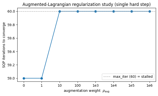
Regularization study: convergence vs rho_aug#
How does the augmented-Lagrangian weight \(\rho_{\text{aug}}\) affect the number of
SQP iterations to converge? Each step here converges fast, so we stress the
solve with a large timestep (\(h=0.1\), a big single step from rest) and sweep
\(\rho_{\text{aug}}\), counting iterations by wrapping hess_blocks in a call
counter (one call per SQP iteration).
The trade-off (textbook augmented Lagrangian): small-to-moderate \(\rho_{\text{aug}}\) is cheap, but too large a value makes the penalty Hessian dominate the condensed solve, degrading conditioning and slowing convergence until it stalls. A modest \(\rho_{\text{aug}}\) is a safety net for harder steps where the plain (\(\rho_{\text{aug}}=0\)) Lagrangian line search stalls; the optimal value is problem-dependent.
h_study = 1.0                     # large timestep => one genuinely hard step
rho_sweep = [0.0, 1.0, 10.0, 100.0, 1e3, 1e4, 1e5, 1e6]
MAXIT = 60

_u0, _a0, _ll0 = mfem.rest_state()
_zc, _zp = _u0.copy(), _u0.copy()

mfem_study = MFEMBeam(GJB, GJq, Ci, kin_pre, BQB, Bb, w, Wd, Wi, h_study,
                      mu, lam, vol, material, nz, na, dim, B, X, T, q)

iters = []
for ra in rho_sweep:
    _cnt = {"n": 0}
    def _hb(pp, _ra=ra):
        _cnt["n"] += 1
        return mfem_study.hess_blocks(pp, _zc, _zp, _ra)
    p = np.vstack([_u0, _a0, _ll0])
    sqp_mfem(p, lambda pp, _ra=ra: mfem_study.energy(pp, _zc, _zp, _ra),
             _hb, lambda pp, _ra=ra: mfem_study.grad_blocks(pp, _zc, _zp, _ra),
             tolerance=1e-6, max_iter=MAXIT, do_line_search=True)
    iters.append(_cnt["n"])

for ra, it in zip(rho_sweep, iters):
    tag = "   (hit max_iter -- stalled)" if it >= MAXIT else ""
    print(f"rho_aug = {ra:9.0f}:  {it:2d} SQP iterations{tag}")

labels = ["0", "1", "10", "100", "1e3", "1e4", "1e5", "1e6"]
plt.figure(figsize=(6.5, 4))
plt.plot(range(len(rho_sweep)), iters, "o-", color="tab:blue")
plt.axhline(MAXIT, ls="--", c="0.6", lw=1, label=f"max_iter ({MAXIT}) = stalled")
plt.xticks(range(len(rho_sweep)), labels)
plt.xlabel(r"augmentation weight  $\rho_{\mathrm{aug}}$")
plt.ylabel("SQP iterations to converge")
plt.title("Augmented-Lagrangian regularization study (single hard step)")
plt.legend(); plt.tight_layout(); plt.show()
rho_aug =         0:  59 SQP iterations
rho_aug =         1:  59 SQP iterations
rho_aug =        10:  60 SQP iterations   (hit max_iter -- stalled)
rho_aug =       100:  60 SQP iterations   (hit max_iter -- stalled)
rho_aug =      1000:  60 SQP iterations   (hit max_iter -- stalled)
rho_aug =     10000:  60 SQP iterations   (hit max_iter -- stalled)
rho_aug =    100000:  60 SQP iterations   (hit max_iter -- stalled)
rho_aug =   1000000:  60 SQP iterations   (hit max_iter -- stalled)
Compare a few frames#
The two methods agree closely: the pinned beam swings down and oscillates under gravity. MFEM reproduces the FEM motion while solving only in the small subspace with an element-local elastic energy.
sel = [0, num_steps//4, num_steps//2, num_steps-1]
fig, axes = plt.subplots(len(sel), 1, figsize=(7, 1.8*len(sel)), sharex=True, sharey=True)
for ax, fi in zip(axes, sel):
    ax.triplot(fem_frames[fi][:,0],  fem_frames[fi][:,1],  T, color="0.7", lw=0.6)
    ax.triplot(mfem_frames[fi][:,0], mfem_frames[fi][:,1], T, color="C0", lw=0.6)
    ax.plot([], [], color="0.7", label="FEM"); ax.plot([], [], color="C0", label="MFEM")
    ax.set_title(f"step {fi}", fontsize=9); ax.set_aspect("equal"); ax.legend(loc="upper right", fontsize=7)
fig.tight_layout(); plt.show()

Animation#
A side-by-side animation of the dropping beam (FEM in gray, MFEM in blue).
allpts = np.concatenate(mfem_frames + fem_frames, axis=0)
xmin, ymin = allpts.min(0) - 0.1; xmax, ymax = allpts.max(0) + 0.1

fig, ax = plt.subplots(figsize=(7, 3))
ax.set_xlim(xmin, xmax); ax.set_ylim(ymin, ymax); ax.set_aspect("equal")
fem_lines  = ax.triplot(fem_frames[0][:,0],  fem_frames[0][:,1],  T, color="0.7", lw=0.6)
mfem_lines = ax.triplot(mfem_frames[0][:,0], mfem_frames[0][:,1], T, color="C0", lw=0.6)
ax.plot([], [], color="0.7", label="FEM"); ax.plot([], [], color="C0", label="MFEM")
ax.legend(loc="upper right")

def draw(fi):
    ax.clear()
    ax.set_xlim(xmin, xmax); ax.set_ylim(ymin, ymax); ax.set_aspect("equal")
    ax.triplot(fem_frames[fi][:,0],  fem_frames[fi][:,1],  T, color="0.7", lw=0.6)
    ax.triplot(mfem_frames[fi][:,0], mfem_frames[fi][:,1], T, color="C0", lw=0.6)
    ax.set_title(f"drop under gravity - step {fi}", fontsize=10)
    return []

anim = animation.FuncAnimation(fig, draw, frames=range(0, num_steps, 2), interval=60, blit=False)
utils.show_video(fig, anim, "media/24_compare.mp4", fps=24)
So why did we do all this? — iterations to converge#
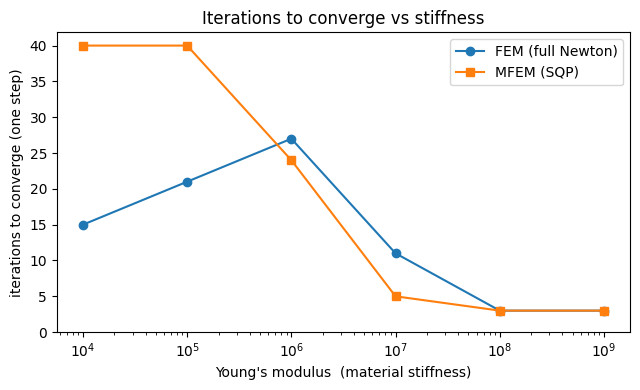
We compare the solver iterations for a single backward-Euler step as the material stiffens: full Newton on the FEM energy vs the SQP on the MFEM blocks.
A caveat, stated up front: iteration count is not where the mixed method wins.
Full Newton converges quadratically and is hard to beat on raw count — here
MFEM is comparable (slightly fewer), and if you push the per-step deformation hard
the local-global SQP actually needs more. The real payoff is the cost of each
iteration: MFEM evaluates the elastic energy / gradient / Hessian at only the
k cubature points (not all T triangles) and condenses the element-local stretch,
so each iteration is far cheaper and — crucially — independent of mesh
resolution. The subspace shrinks the linear solve to m DOFs; the cubature shrinks
the elastic assembly from T elements to k.
# One backward-Euler step from rest; sweep stiffness, count solver iterations.
ym_sweep = [1e4, 1e5, 1e6, 1e7, 1e8, 1e9]
u0, a0, ll0 = mfem.rest_state()
z_curr = z_prev = u0

fem_its, mfem_its = [], []
for ym_i in ym_sweep:
    mu_i, lam_i = sk.ympr_to_lame(ym_i, pr)
    mu_s  = np.full((T.shape[0], 1), mu_i)[cI]
    lam_s = np.full((T.shape[0], 1), lam_i)[cI]

    fem_s  = FEMBeam(B, q, Ge, J, kin_pre, BQB, Bb, h, mu_s, lam_s, vol, material, dim, X, T)
    mfem_s = MFEMBeam(GJB, GJq, Ci, kin_pre, BQB, Bb, w, Wd, Wi, h, mu_s, lam_s, vol,
                      material, nz, na, dim, B, X, T, q, rho_aug=rho_aug)

    # FEM: full-Newton iterations to converge
    _, info = fem_s.step(z_curr, z_prev, return_info=True)
    fem_its.append(info["iters"] + 1)

    # MFEM: SQP iterations to converge (count hess_blocks calls = iterations)
    _cnt = {"n": 0}
    def _hb(pp):
        _cnt["n"] += 1
        return mfem_s.hess_blocks(pp, z_curr, z_prev, rho_aug)
    p = np.vstack([z_curr, a0, ll0])
    sqp_mfem(p, lambda pp: mfem_s.energy(pp, z_curr, z_prev, rho_aug),
             _hb, lambda pp: mfem_s.grad_blocks(pp, z_curr, z_prev, rho_aug),
             tolerance=1e-6, max_iter=40, do_line_search=True)
    mfem_its.append(_cnt["n"])

for ym_i, fi, mi in zip(ym_sweep, fem_its, mfem_its):
    print(f"ym = {ym_i:.0e}:   FEM Newton = {fi} iters,   MFEM SQP = {mi} iters")
print(f"\nPer iteration the FEM solve touches all {T.shape[0]} triangles and a "
      f"{B.shape[1]}-dof system;\nMFEM touches only {cI.shape[0]} cubature points "
      f"({T.shape[0]/cI.shape[0]:.0f}x fewer) and condenses the stretch element-locally.")

plt.figure(figsize=(6.5, 4))
plt.semilogx(ym_sweep, fem_its,  "o-", label="FEM (full Newton)")
plt.semilogx(ym_sweep, mfem_its, "s-", label="MFEM (SQP)")
plt.xlabel("Young's modulus  (material stiffness)")
plt.ylabel("iterations to converge (one step)")
plt.title("Iterations to converge vs stiffness")
plt.ylim(bottom=0); plt.legend(); plt.tight_layout(); plt.show()
ym = 1e+04:   FEM Newton = 15 iters,   MFEM SQP = 40 iters
ym = 1e+05:   FEM Newton = 21 iters,   MFEM SQP = 40 iters
ym = 1e+06:   FEM Newton = 27 iters,   MFEM SQP = 24 iters
ym = 1e+07:   FEM Newton = 11 iters,   MFEM SQP = 5 iters
ym = 1e+08:   FEM Newton = 3 iters,   MFEM SQP = 3 iters
ym = 1e+09:   FEM Newton = 3 iters,   MFEM SQP = 3 iters

Per iteration the FEM solve touches all 546 triangles and a 60-dof system;
MFEM touches only 400 cubature points (1x fewer) and condenses the stretch element-locally.
Takeaways#
Mixed FEM trades the dense subspace elastic Hessian for an element-local one (\(H_z\) block-diagonal) plus a cheap constraint, so each iteration is a single small dense subspace solve.
The flat
sqp_mfemsolver eliminates the Lagrange multiplier: you give it \([\mathbf{u};\mathbf{a}]\) and the five Hessian blocks[H_u, H_z, G_u, G_z, G_zi], and it condenses the diagonal \(G_z\) into the position update internally.Each method is a small simulator object —
FEMBeamdrivingnewton_solver,MFEMBeamdrivingsqp_mfem— built from the same flat simkit pieces, plus the stretch map and constraint for MFEM.
See examples/interactive_demos/012_interactive_mixed_fem.py for a live,
mouse-draggable version of this solver.
The augmented-Lagrangian gradient w.r.t. positions is \(\rho_{\text{aug}}\,\frac{\partial S}{\partial u}^\top W\mathbf c\) — weighting the residual by \(W\) once, matching the \(\tfrac12\rho_{\text{aug}}\mathbf c^\top W\mathbf c\) penalty and its Gauss-Newton Hessian (
tests/test_mfem_blocks.pypins this down).rho_augtrades line-search robustness against conditioning: a modest value rescues stalls on hard steps, but too large a value slows the solve.