25 · Modal Muscle Actuation#

How does a soft creature move itself? Not with an artist painting muscle fibers, and not with a hand-rigged skeleton — but with its own natural vibration modes, used as actuators.

This is the idea behind Modal Muscles / Actuators à la Mode (Benchekroun et al.):

A reduced skinning-eigenmode subspace \(B\) carries the deformation, with a handful of reduced coordinates \(\mathbf{z}\) so that \(\mathbf{x} = B\,\mathbf{z}\).
A small set of displacement modes \(D\) — obtained for free from a linear modal analysis of the shape — act as muscles. Dialing each muscle’s amplitude \(a_i\) drives a clustered plastic stretch tensor: a per-element rest target that the flesh tries to match, while passive ARAP elasticity and inertia resist.
No painted muscles, no user rig, no training data. The actuation space is the shape’s own modal space.

We will:

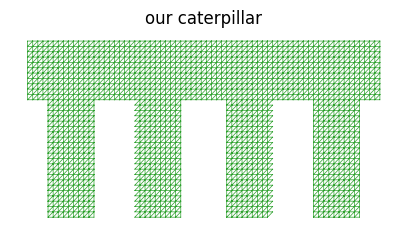
Build a 2D caterpillar creature (four legs, fully triangulated).
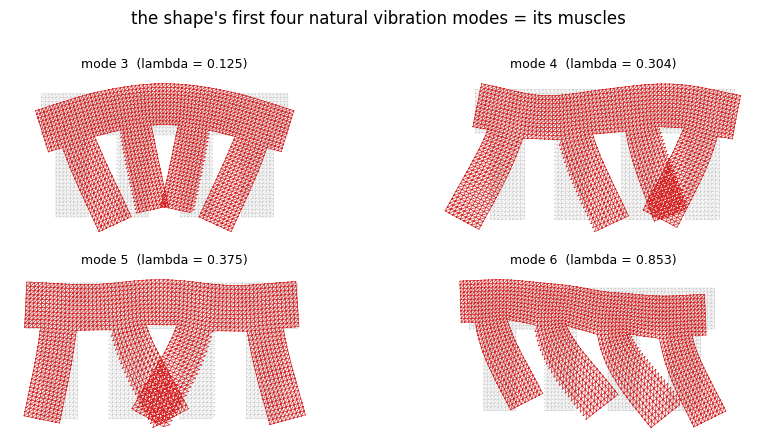
Ask how does it naturally move? → linear modal analysis, dropping the rigid modes.
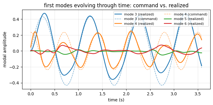
Treat those modes as muscles and float the creature in gravity-free space, contrasting the kinematic actuation target (left) against the inertial simulation (right), and plotting how the modes evolve in time.
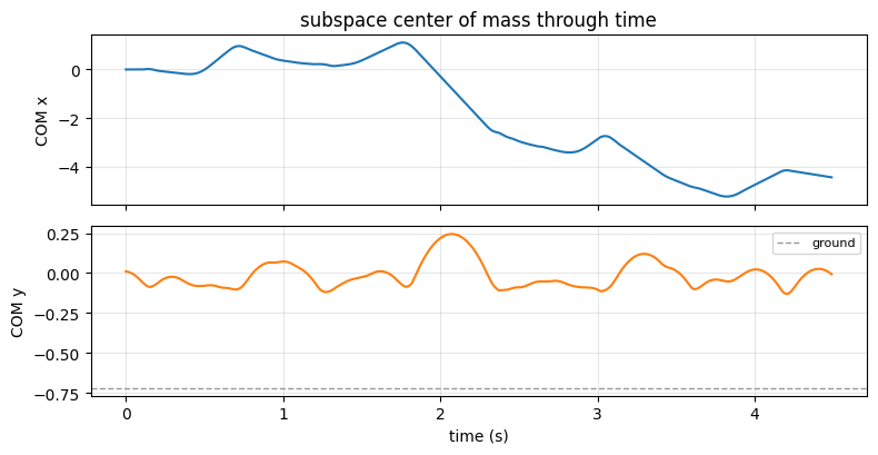
Drop it under gravity with contact and wiggle its muscles into a gait, tracking the center of mass as it crawls.

The whole modal-muscle solver lives in one standardized simulator class, ModalMuscle, built from flat simkit functions. The interactive counterpart is examples/interactive_demos/014_modal_muscles.py.

%matplotlib inline
import numpy as np
import scipy as sp
import scipy.sparse as sps
import matplotlib.pyplot as plt
from matplotlib import animation

import simkit as sk
from simkit.clustered_plastic_stretch_tensor import clustered_plastic_stretch_tensor
from simkit.fast_sandwich_transform_clustered import fast_sandwich_transform_clustered
from simkit.solvers import block_coord
import utils

# sparse @ on some scipy/numpy combos emits spurious 'divide by zero in matmul'
# warnings; the arithmetic is exact. Silence them for a clean notebook.
import warnings; warnings.filterwarnings("ignore")
np.seterr(all="ignore")

{'divide': 'warn', 'over': 'warn', 'under': 'ignore', 'invalid': 'warn'}

A creature, not a rectangle#

We build a little caterpillar: a horizontal body bar with four stubby legs. Rather than load a mesh from disk, we triangulate it from scratch — lay a regular triangle grid over a bounding box and keep only the triangles whose centroid falls inside the body bar or one of the four legs. Dropping the unused vertices leaves a single watertight, conforming triangle mesh.

def caterpillar_mesh(nx=70, ny=34, W=4.0, H=2.0,
                     body_frac=0.34, n_legs=4, leg_frac=0.5):
    # A staple-/caterpillar-shaped triangle mesh: a body bar + n_legs legs.
    # body_frac: fraction of the height taken by the top bar.
    # leg_frac:  total fraction of the width occupied by the legs.
    xs = np.linspace(0, W, nx); ys = np.linspace(0, H, ny)
    XX, YY = np.meshgrid(xs, ys, indexing="xy")
    X = np.stack([XX.ravel(), YY.ravel()], axis=1)
    i, j = np.meshgrid(np.arange(nx - 1), np.arange(ny - 1), indexing="xy")
    v00 = (j*nx + i).ravel();     v01 = (j*nx + i + 1).ravel()
    v10 = ((j+1)*nx + i).ravel(); v11 = ((j+1)*nx + i + 1).ravel()
    T = np.stack([np.stack([v00, v01, v11], 1),
                  np.stack([v00, v11, v10], 1)], 1).reshape(-1, 3)

    c = X[T].mean(1)                       # triangle centroids
    body_y0 = H * (1 - body_frac)
    in_body = c[:, 1] >= body_y0           # the top bar
    leg_w = W * leg_frac / n_legs
    span = W / n_legs
    in_leg = np.zeros(len(c), bool)
    for k in range(n_legs):                # four legs hanging below the bar
        cx = span * (k + 0.5)
        in_leg |= (np.abs(c[:, 0] - cx) <= leg_w / 2) & (c[:, 1] < body_y0)

    Tk = T[in_body | in_leg]
    used = np.unique(Tk)                   # drop vertices no triangle references
    remap = -np.ones(X.shape[0], int); remap[used] = np.arange(len(used))
    return X[used], remap[Tk]

X, T = caterpillar_mesh()
X = sk.normalize_and_center(X)             # center at origin, unit-ish scale
n, dim = X.shape
print(f"{n} vertices, {T.shape[0]} triangles")

fig, ax = plt.subplots(figsize=(5, 2.6))
ax.triplot(X[:, 0], X[:, 1], T, color="C2", lw=0.5)
ax.set_aspect("equal"); ax.set_title("our caterpillar"); ax.axis("off")
plt.show()

1719 vertices, 3058 triangles

../_images/9812c8aa690156f1f3d7eaea57c76895a2e7af7b7abe771d7265965aca4cecb8.png

How does this shape naturally move?#

Pluck the creature and let it ring. The motions it settles into are its natural vibration modes — the eigenvectors of the generalized eigenproblem \(K\,\mathbf{d} = \lambda\, M\,\mathbf{d}\), where \(K\) is the elastic stiffness and \(M\) is the mass matrix. sk.linear_modal_analysis returns them ordered by eigenvalue (frequency²).

The lowest few eigenvalues are essentially zero: those are the rigid modes — ways the shape can move without deforming at all. In 2D there are exactly three (two translations + one rotation). They carry no elastic energy, so they make useless muscles; we drop them and keep the first genuine deformation modes that follow.

n_keep = 4                                   # how many real deformation modes we want
n_rigid = 3                                  # 2 translations + 1 rotation (2D)
E, D = sk.linear_modal_analysis(X, T, n_rigid + n_keep)
modeset = list(range(n_rigid, n_rigid + n_keep))   # [3, 4, 5, 6]

print("eigenvalues (frequency^2):")
for i, e in enumerate(E):
    tag = "  <- rigid (approx 0)" if i < n_rigid else "  <- muscle mode"
    print(f"  mode {i}:  {e: .4e}{tag}")

eigenvalues (frequency^2):
  mode 0:  -3.6066e-13  <- rigid (approx 0)
  mode 1:  -7.2885e-14  <- rigid (approx 0)
  mode 2:   3.3790e-13  <- rigid (approx 0)
  mode 3:   1.2494e-01  <- muscle mode
  mode 4:   3.0425e-01  <- muscle mode
  mode 5:   3.7463e-01  <- muscle mode
  mode 6:   8.5344e-01  <- muscle mode

The first four muscle modes#

Each surviving mode is a whole-body deformation field. Below we visualize them by pushing the rest shape along each mode. These four fields are our entire muscle vocabulary — obtained automatically, with no rig and no painted fibers.

# a per-mode visual amplitude so each mode displaces a comparable, visible amount
scale = 0.35 / np.abs(D[:, modeset]).max(0)

fig, axes = plt.subplots(2, 2, figsize=(9, 4.4))
for ax, mi, sc in zip(axes.ravel(), modeset, scale):
    dvec = D[:, mi].reshape(n, dim)
    ax.triplot(X[:, 0], X[:, 1], T, color="0.82", lw=0.4)          # rest
    Xp = X + sc * dvec
    ax.triplot(Xp[:, 0], Xp[:, 1], T, color="C3", lw=0.5)          # actuated
    ax.set_aspect("equal"); ax.axis("off")
    ax.set_title(f"mode {mi}  (lambda = {E[mi]:.3f})", fontsize=9)
fig.suptitle("the shape's first four natural vibration modes = its muscles", y=1.0)
fig.tight_layout(); plt.show()

../_images/82650f13b695ce0e644f3bf52e940af40794b0a80e2590bdc64b88f925f7e751.png

Modal muscles, in one paragraph#

We keep two reduced spaces over the same mesh:

Subspace \(B\) — skinning eigenmodes (sk.skinning_eigenmodes), mass-orthonormalized. The simulation only ever solves for the reduced state \(\mathbf{z}\), with \(\mathbf{x} = B\,\mathbf{z}\). This is what makes it fast.
Muscles \(D\) — the linear modes we just found, plus the rest pose as a final column so the activation vector \(\mathbf{a}\) can encode “stay at rest”. Activating \(\mathbf{a}\) defines, per element, a target plastic stretch the material wants to assume.

Each timestep alternates two cheap steps (simkit.solvers.block_coord):

local step — per cluster of elements, a polar_svd gives the best-fit rotation for the passive ARAP energy and for the active clustered plastic-stretch target \(K(\mathbf{z}, \mathbf{a})\).
global step — one Cholesky back-solve in the subspace \(B\) that balances passive elasticity, the active muscle pull, inertia, and (later) contact.

The next cell is the whole solver, packed into a single standardized simulator class, ModalMuscle. Its __init__ runs all the precompute once (subspace operators, muscle operators, clusters, reduced mass, the Cholesky factorization, optional contact operators, and the constant gravity force \(b_0\)); from then on we only call rest_state() and step(z, z_dot, a). The local_step / global_step pieces are kept as named methods so you can read the passive (ARAP) and active (muscle) energy contributions where they enter the global solve.

class ModalMuscle:
    """Reduced modal-muscle dynamics: x = B z, muscles drive a clustered plastic
    stretch target while passive ARAP elasticity + inertia (+ optional contact)
    resist. One local/global block_coord solve per step, all inside subspace B."""

    def __init__(self, X, T, B, D, l, d, *, mu=1e6, gamma=1e6, rho=1e3, h=1e-2,
                 b0=None, contact=False, cI=None, plane_pos=None,
                 alpha=1.0, max_iter=10, tolerance=1e-6):
        # B : (dim*n, r) skinning-eigenmode subspace; reduced state z, x = B z.
        # D : (dim*n, m) muscle (displacement) modes; activation a (m,1).
        # l : passive cubature cluster labels;  d : active cluster labels.
        # mu, gamma : passive / active stiffness;  b0 : constant reduced force.
        dim, nT = X.shape[1], T.shape[0]
        l = l.astype(int); d = d.astype(int)
        self.dim, self.h, self.alpha = dim, h, alpha
        self.max_iter, self.tolerance = max_iter, tolerance
        self.B, self.D, self.contact = B, D, contact

        vol = sk.volume(X, T)
        J = sk.deformation_jacobian(X, T)
        Mv = sps.kron(sk.massmatrix(X, T, rho=rho), sps.identity(dim))
        self.Mv = Mv

        # ---- passive ARAP, grouped into clusters ----
        mu_v, gamma_v = np.full((nT, 1), mu), np.full((nT, 1), gamma)
        P, _ = sk.cluster_grouping_matrices(l, X, T)
        A = sps.diags(vol.flatten())
        AMue  = sps.kron(A @ sps.diags(mu_v.flatten()),       sps.identity(dim * dim))
        PAMue = sps.kron(P @ (A @ sps.diags(mu_v.flatten())), sps.identity(dim * dim))
        self.AMuPJB = (PAMue @ J) @ B
        L_passive = J.T @ AMue @ J

        # ---- active muscle force (clustered plastic stretch tensor) ----
        AGammae = sps.kron(A @ sps.diags(gamma_v.flatten()), sps.identity(dim * dim))
        L_active = J.T @ AGammae @ J
        BJAgamma = B.T @ (J.T @ AGammae)
        self.K   = clustered_plastic_stretch_tensor(X, T, d, B, D, w=(vol * gamma_v).reshape(-1, 1))
        self.fst = fast_sandwich_transform_clustered(BJAgamma, J @ D, d, dim=dim)

        # ---- reduced mass, stiffness operators, projection bases ----
        self.BMB = B.T @ Mv @ B
        self.BMy = B.T @ Mv @ X.reshape(-1, 1)
        self.DMD = D.T @ Mv @ D
        self.DMy = D.T @ Mv @ X.reshape(-1, 1)

        # ---- system Hessian + Cholesky factorization ----
        H = B.T @ L_passive @ B + B.T @ L_active @ B + self.BMB / h**2
        self.chol_H = sp.linalg.cho_factor(H)
        self.b = np.zeros((B.shape[1], 1)) if b0 is None else b0.reshape(-1, 1)

        self.num_passive_clusters = int(l.max()) + 1
        self.num_active_clusters  = int(d.max()) + 1

        # ---- optional ground-plane contact ----
        if contact:
            if plane_pos is None:
                plane_pos = np.zeros((dim, 1))
            Se = sps.kron(sk.selection_matrix(np.unique(cI), X.shape[0]), sps.identity(dim))
            self.plane_pos = plane_pos
            self.Je = Se @ B
            self.JeQi = sp.linalg.cho_solve(self.chol_H, self.Je.T).T

    def rest_state(self, X):
        # Reduced rest state (z, z_dot, a) projected from the rest pose X.
        z = sk.project_into_subspace(X.reshape(-1, 1), self.B, M=self.Mv, BMB=self.BMB, BMy=self.BMy)
        a = sk.project_into_subspace(X.reshape(-1, 1), self.D, M=self.Mv, BMB=self.DMD, BMy=self.DMy)
        return z, np.zeros_like(z), a

    def _contact_projection(self, z, f, z_curr):
        # Velocity-level ground-plane contact, in the spirit of projective
        # dynamics, folded into the global solve: any contact point below the
        # plane AND moving into it gets its downward velocity removed.
        dim, h, alpha = self.dim, self.h, self.alpha
        Je, JeQi, plane_pos = self.Je, self.JeQi, self.plane_pos
        z_dot_tent = (sp.linalg.cho_solve(self.chol_H, f) - z_curr) / h
        Pp = (Je @ z).reshape(-1, dim)
        under = (Pp[:, 1] < plane_pos[1]).flatten()
        local_vel = (Je @ z_dot_tent).reshape(-1, dim)
        ci = np.where(under & (local_vel[:, 1] < 0))[0]
        if ci.shape[0] == 0:
            return np.zeros_like(f)
        idx = (np.repeat(ci[:, None], dim, 1) * dim + np.arange(dim)).flatten()
        JeI, L = Je[idx, :], JeQi[idx, :]
        v = np.zeros((ci.shape[0], dim)); v[:, 0] = (1.0 - alpha) * local_vel[ci, 0]
        p = (JeI @ z_curr).reshape(-1, dim)
        bb = (v * h + p - (L @ f).reshape(-1, dim)).reshape(-1, 1)
        if L.shape[0] >= L.shape[1]:
            return np.linalg.solve(L.T @ L, L.T @ bb)
        return L.T @ np.linalg.solve(L @ L.T, bb)

    def local_step(self, zc, a):
        # best-fit rotations: passive ARAP + active clustered plastic stretch
        R_p = sk.polar_svd((self.AMuPJB @ zc).reshape(-1, self.dim, self.dim))[0]
        R_a = sk.polar_svd(self.K(zc, a))[0]
        return np.vstack([R_p.reshape(-1, 1), R_a.reshape(-1, 1)])

    def global_step(self, zc, r, a, k, z_curr):
        # one Cholesky solve in the subspace, summing the reduced forces
        dim = self.dim
        pd = self.num_passive_clusters * dim**2
        ad = self.num_active_clusters * dim**2
        E_inertia = k                                          # inertial target
        E_passive = self.AMuPJB.T @ r[:pd]                    # passive ARAP pull
        E_active  = self.fst(r[pd:pd + ad].reshape(-1, dim, dim)) @ a  # muscle pull
        f = E_inertia + E_passive + E_active - self.b
        if self.contact:
            contact = self._contact_projection(zc, f, z_curr)  # ground-plane push
            f = f + contact
        return sp.linalg.cho_solve(self.chol_H, f)

    def step(self, z, z_dot, a):
        # Advance one timestep; return the next reduced state z_next.
        h = self.h
        k = self.BMB @ (z + h * z_dot) / h**2                 # inertial target
        z_curr = z.copy()
        local  = lambda zc: self.local_step(zc, a)
        glob   = lambda zc, r: self.global_step(zc, r, a, k, z_curr)
        return block_coord(z.copy(), glob, local,
                           tolerance=self.tolerance, max_iter=self.max_iter)

Building the reduced model#

We assemble the three reduced ingredients once:

B — the skinning-eigenmode subspace, mass-orthonormalized.
Dms — our four muscle modes, with the rest pose appended as a final column (so the activation can hold the rest state).
l — spectral cubature cluster labels, grouping the triangles into a handful of clusters so the local step is cheap.

limit_a is a per-mode amplitude ceiling from sk.limit_actuation_dirichlet_energy: how hard we can pull a muscle before the plastic target becomes unreasonably stretched. We scale all our sinusoids by it.

num_modes  = 8     # skinning-eigenmode subspace dimension
num_clust  = 20    # cubature clusters for the passive local step

Wmd, _E, B = sk.skinning_eigenmodes(X, T, num_modes)
B = sk.orthonormalize(B, M=sps.kron(sk.massmatrix(X, T), sps.identity(dim)))

# muscles = the 4 deformation modes + rest pose (so activation can encode "rest")
Dms = np.hstack([D[:, modeset], X.reshape(-1, 1)])

# cubature: group triangles into clusters for the clustered local/global steps
_cI, _cW, l = sk.spectral_cubature(X, T, Wmd, num_clust, return_labels=True)
d = np.zeros(T.shape[0])                       # a single active cluster

limit_a = sk.limit_actuation_dirichlet_energy(X, T, D, max_s=2.0)[modeset]
print(f"subspace dim = {B.shape[1]},  muscles = {len(modeset)},  clusters = {num_clust}")
print("per-muscle amplitude ceiling:", np.round(limit_a, 3))

subspace dim = 48,  muscles = 4,  clusters = 20
per-muscle amplitude ceiling: [0.48  0.394 0.298 0.248]

Floating in space: actuation target vs. inertial response#

First, no gravity and no ground — the creature floats in 2D, driven only by its muscles and its own inertia. We wiggle the first two muscles sinusoidally.

To see what the simulation is doing, we show two things side by side:

left (the actuation target): the purely kinematic shape the muscles ask for,

\[ \mathbf{x}_{\text{target}} = \mathbf{x}_{\text{rest}} + \sum_i a_i(t)\,D_i . \]

This is the muscle command — instantaneous and weightless.
right (the simulation): the actual reduced dynamics \(\mathbf{x} = B\,\mathbf{z}\), where inertia and passive elasticity lag and smooth that command.

A floating body conserves momentum, so it can change its shape freely but its center of mass barely moves — the muscles let it “swim in place”.

# --- a gravity-free, contact-free modal-muscle sim ---
sim_float = ModalMuscle(X, T, B, Dms, l, d,
                        mu=1e5, gamma=1e5, rho=1e3, h=0.02, max_iter=10)
h = sim_float.h
n_steps = 180

# sinusoidal muscle command: amplitude (x limit_a), period (s), phase (x period)
amp_float    = np.array([0.9, 0.6, 0.0, 0.0]) * limit_a
period_float = np.array([1.0, 0.7, 1.0, 1.0])
phase_float  = np.array([0.0, 0.25, 0.0, 0.0])

def activation_float(t):
    return amp_float * np.sin(2 * np.pi * (t / period_float + phase_float))

# operators to read off the realized modal amplitude of the *simulation*
Dm   = D[:, modeset]
DmM  = Dm.T @ sim_float.Mv                        # (4, dim*n)
DmMD = np.diag(Dm.T @ sim_float.Mv @ Dm)         # (4,)
xrest = X.reshape(-1, 1)

z, z_dot, a = sim_float.rest_state(X)
sim_frames, tgt_frames, a_input, a_realized = [], [], [], []
for i in range(n_steps):
    t = i * h
    a_t = activation_float(t)
    a[:-1, 0] = a_t                               # last entry holds the rest column
    z_next = sim_float.step(z, z_dot, a)
    z_dot = (z_next - z) / h
    z = z_next.copy()

    x_sim = (B @ z)                               # simulated positions
    sim_frames.append(x_sim.reshape(n, dim))
    tgt_frames.append((xrest + Dm @ a_t.reshape(-1, 1)).reshape(n, dim))
    a_input.append(a_t)
    a_realized.append(((DmM @ (x_sim - xrest)).flatten() / DmMD))

a_input    = np.array(a_input)
a_realized = np.array(a_realized)
print("floated", n_steps, "steps")

floated 180 steps

Side by side: command (left) vs. simulation (right)#

allpts = np.concatenate(sim_frames + tgt_frames, 0)
lo = allpts.min(0) - 0.15; hi = allpts.max(0) + 0.15

fig, (axL, axR) = plt.subplots(1, 2, figsize=(10, 3.2))
def draw_float(fi):
    for ax, frames, title, col in [(axL, tgt_frames, "actuation target  x = X + sum a_i D_i", "C3"),
                                   (axR, sim_frames, "simulation  x = B z", "C0")]:
        ax.clear()
        ax.triplot(frames[fi][:, 0], frames[fi][:, 1], T, color=col, lw=0.5)
        ax.set_xlim(lo[0], hi[0]); ax.set_ylim(lo[1], hi[1])
        ax.set_aspect("equal"); ax.axis("off"); ax.set_title(title, fontsize=10)
    return []

anim = animation.FuncAnimation(fig, draw_float, frames=range(0, n_steps, 3),
                               interval=60, blit=False)
utils.show_video(fig, anim, "media/25_floating.mp4", fps=24)

How the modes evolve through time#

The muscle command is a clean sinusoid (dashed). The body’s realized modal amplitude (solid) — the projection of the actual simulated motion onto each linear mode — lags and rounds it off: that is inertia and passive stiffness filtering the command. Undriven modes (2 and 3) stay near zero, but pick up a little energy through nonlinear coupling.

fig, ax = plt.subplots(figsize=(8, 3.4))
ts = np.arange(n_steps) * h
colors = ["C0", "C1", "C2", "C3"]
for j, mi in enumerate(modeset):
    ax.plot(ts, a_realized[:, j], color=colors[j], lw=1.8, label=f"mode {mi} (realized)")
    if amp_float[j] != 0:
        ax.plot(ts, a_input[:, j], color=colors[j], lw=1.0, ls="--", alpha=0.7,
                label=f"mode {mi} (command)")
ax.set_xlabel("time (s)"); ax.set_ylabel("modal amplitude")
ax.set_title("first modes evolving through time: command vs. realized")
ax.legend(fontsize=8, ncol=2, loc="upper right"); ax.grid(alpha=0.3)
plt.show()

../_images/5bce627e1b80f56bfc9d309924918d40f5ddbe27dd40d577285257ffdabe5a81.png

Now let it fall, and let it crawl#

Time to put the caterpillar on the ground. We rebuild the sim with two additions:

gravity — a constant reduced force \(-B^\top \mathbf{g}\).
contact — a velocity-level ground plane, in the spirit of projective dynamics: at each global solve, every boundary contact point that is below the plane and moving into it has its into-the-ground velocity removed (_contact_projection). Tangential sliding is preserved, so pushing legs against the floor produces forward thrust.

Contact points are a handful of boundary vertices (found by keeping mesh edges that belong to a single triangle, then farthest-point sampling). We place the floor just below the creature so it drops, lands, and then crawls under muscle power.

def boundary_vertices(T):
    # vertices on edges that belong to exactly one triangle
    e = np.sort(np.vstack([T[:, [0, 1]], T[:, [1, 2]], T[:, [2, 0]]]), axis=1)
    uniq, cnt = np.unique(e, axis=0, return_counts=True)
    return np.unique(uniq[cnt == 1])

bv = boundary_vertices(T)
cI = bv[sk.farthest_point_sampling(X[bv, :], 30)]    # contact sample points
ground_y = float(X[:, 1].min()) - 0.15               # floor just below the feet

g = B.T @ sk.gravity_force(X, T, a=-9.8, rho=1e3).reshape(-1, 1)
sim_grav = ModalMuscle(X, T, B, Dms, l, d,
                       mu=1e6, gamma=1e6, rho=1e3, h=1e-2,
                       b0=-g, contact=True, cI=cI,
                       plane_pos=np.array([[0.0], [ground_y]]), alpha=1.0,
                       max_iter=10)
print(f"{cI.shape[0]} contact points,  ground at y = {ground_y:.3f}")

30 contact points,  ground at y = -0.720

Dial in a gait#

These four lines are the knobs — edit them and re-run to invent new gaits. Each muscle gets an amplitude (as a fraction of its ceiling), a period (seconds), and a phase (fraction of a period). Phase offsets between the legs are what break symmetry and turn a wiggle into directed crawling.

# ----------------------- EDIT ME: the gait -----------------------
amp_frac = np.array([0.45, 0.35, 0.25, 0.15])   # per-muscle amplitude (x ceiling)
periods  = np.array([1.20, 0.80, 1.00, 0.60])   # seconds per cycle
phases   = np.array([0.00, 0.25, 0.50, 0.10])   # fraction of a period
# -----------------------------------------------------------------
n_steps_g = 450
hg = sim_grav.h
amp_g = amp_frac * limit_a

def activation_gait(t):
    return amp_g * np.sin(2 * np.pi * (t / periods + phases))

# cached center-of-mass operator (subspace COM): com(t) = subspace_com(z_t, ...)
_com0, SB = sk.subspace_com(np.zeros(B.shape[1]), B, X, T, return_SB=True)

z, z_dot, a = sim_grav.rest_state(X)
crawl_frames, com = [], []
for i in range(n_steps_g):
    t = i * hg
    a[:-1, 0] = activation_gait(t)
    z_next = sim_grav.step(z, z_dot, a)
    z_dot = (z_next - z) / hg
    z = z_next.copy()
    crawl_frames.append((B @ z).reshape(n, dim))
    com.append(sk.subspace_com(z.flatten(), B, X, T, SB=SB).flatten())

com = np.array(com)
print(f"crawled {n_steps_g} steps")
print(f"horizontal COM travel: {com[-1, 0] - com[0, 0]:+.3f}")
print(f"vertical COM range:    [{com[:,1].min():.3f}, {com[:,1].max():.3f}]  (ground y = {ground_y:.3f})")

crawled 450 steps
horizontal COM travel: -4.438
vertical COM range:    [-0.130, 0.244]  (ground y = -0.720)

Center of mass over time#

The subspace center of mass sk.subspace_com(z, B, X, T) reads the creature’s COM straight from the reduced state. Its horizontal coordinate is our measure of locomotion: a gait that crawls shows steady horizontal drift, with a gentle vertical bob as the legs cycle.

ts_g = np.arange(n_steps_g) * hg
fig, (a1, a2) = plt.subplots(2, 1, figsize=(8, 4.2), sharex=True)
a1.plot(ts_g, com[:, 0], "C0"); a1.set_ylabel("COM x"); a1.grid(alpha=0.3)
a1.set_title("subspace center of mass through time")
a2.plot(ts_g, com[:, 1], "C1"); a2.axhline(ground_y, color="0.6", ls="--", lw=1, label="ground")
a2.set_ylabel("COM y"); a2.set_xlabel("time (s)"); a2.legend(fontsize=8); a2.grid(alpha=0.3)
fig.tight_layout(); plt.show()

../_images/79cf66cddd2d4c266bb64fb09945bd609a2499780af7f156c4356bc9130201f1.png

Watch it crawl#

Left: the caterpillar over the floor (the COM marked with a dot). Right: its horizontal COM position drawn in as time advances — the animated trace of locomotion.

allc = np.concatenate(crawl_frames, 0)
xlo, xhi = allc[:, 0].min() - 0.3, allc[:, 0].max() + 0.3
ylo, yhi = ground_y - 0.1, allc[:, 1].max() + 0.2
stride = 5
sel = range(0, n_steps_g, stride)

fig, (axA, axB) = plt.subplots(1, 2, figsize=(11, 3.4))
def draw_crawl(fi):
    axA.clear()
    axA.fill_between([xlo, xhi], ylo, ground_y, color="0.85")        # the ground
    axA.axhline(ground_y, color="0.5", lw=1)
    axA.triplot(crawl_frames[fi][:, 0], crawl_frames[fi][:, 1], T, color="C2", lw=0.5)
    axA.plot(com[fi, 0], com[fi, 1], "o", color="C3", ms=6)          # COM marker
    axA.set_xlim(xlo, xhi); axA.set_ylim(ylo, yhi); axA.set_aspect("equal")
    axA.set_title(f"crawling under gravity   t = {fi*hg:.2f}s", fontsize=10); axA.axis("off")

    axB.clear()
    axB.plot(ts_g[:fi+1], com[:fi+1, 0], "C0")
    axB.plot(ts_g[fi], com[fi, 0], "o", color="C3", ms=6)
    axB.set_xlim(0, ts_g[-1]); axB.set_ylim(com[:, 0].min() - 0.1, com[:, 0].max() + 0.1)
    axB.set_xlabel("time (s)"); axB.set_ylabel("COM x")
    axB.set_title("horizontal COM position", fontsize=10); axB.grid(alpha=0.3)
    return []

anim = animation.FuncAnimation(fig, draw_crawl, frames=sel, interval=60, blit=False)
utils.show_video(fig, anim, "media/25_crawling.mp4", fps=24)

Takeaways#

A shape’s linear vibration modes (minus the rigid ones) are a ready-made, rig-free set of muscles — no painting, no skeleton, no data.
Modal muscles activate those modes as a clustered plastic stretch target; passive ARAP elasticity and inertia respond, and the whole step is a cheap local/global block_coord solve inside a skinning-eigenmode subspace.
Floating, the muscles reshape the body while momentum pins the COM. On the ground, the same sinusoids — with phase offsets between the legs — turn into a gait, and sk.subspace_com lets us read locomotion straight from the reduced state.
The whole solver is one standardized ModalMuscle class built from flat simkit functions: linear_modal_analysis, skinning_eigenmodes, spectral_cubature, clustered_plastic_stretch_tensor, fast_sandwich_transform_clustered, and solvers.block_coord.

Go back to the gait cell and try your own amplitudes, periods, and phases — or open examples/interactive_demos/014_modal_muscles.py for a live, slider-driven version, and examples/modal_muscles/actuators_a_la_mode_2D.py to see CMA-ES optimize these very parameters for fastest forward crawl.

# Optional: CMA-ES gait optimization (matches actuators_a_la_mode_2D.py).
# Guarded off by default so the notebook never launches a long optimization at
# build time. Flip RUN_CMA = True (and `pip install cma`) to search for the gait
# that maximizes forward COM travel; the budget here is deliberately tiny.
RUN_CMA = False

if RUN_CMA:
    import cma

    def crawl_distance(params):
        amp_f  = np.clip(params[0:4], 0.0, 1.0)
        per    = np.clip(params[4:8], 0.4, 1.5)
        pha    = params[8:12]
        amp_p  = amp_f * limit_a

        z, z_dot, a = sim_grav.rest_state(X)
        for i in range(150):                       # short rollout for the search
            t = i * hg
            a[:-1, 0] = amp_p * np.sin(2 * np.pi * (t / per + pha))
            z_next = sim_grav.step(z, z_dot, a)
            z_dot = (z_next - z) / hg
            z = z_next.copy()
        com_end = sk.subspace_com(z.flatten(), B, X, T, SB=SB).flatten()
        return -(com_end[0] - _com0[0])            # CMA minimizes; we want +x travel

    x0 = np.concatenate([amp_frac, periods, phases])
    es = cma.CMAEvolutionStrategy(x0, 0.2,
                                  {"maxfevals": 24, "popsize": 6, "verbose": -9})
    es.optimize(crawl_distance)
    print("best gait params:", np.round(es.result.xbest, 3))
    print("best forward travel:", round(-es.result.fbest, 4))
else:
    print("CMA-ES disabled (set RUN_CMA = True to optimize the gait).")

CMA-ES disabled (set RUN_CMA = True to optimize the gait).