3 · Elastic Energy Intuition#
The deformation gradient \(F\) says how a triangle is deformed. An elastic energy \(\psi(F)\) turns that into a single number: how much it costs.
We will write each energy out ourselves — one line of math each — so nothing is hidden, then compare three classics:
Linear elasticity
ARAP (as-rigid-as-possible)
Neo-Hookean (classical)
A good energy is zero for rigid motions (translation, rotation) and grows with genuine deformation (scale, shear). We’ll see linear elasticity fail the rotation test, and Neo-Hookean blow up as a triangle is crushed flat.
%matplotlib inline
import numpy as np
import matplotlib.pyplot as plt
import simkit
import utils
The three energies, written out#
All three are functions of \(F\) alone, with material constants \(\mu\) (shear) and \(\lambda\) (bulk). Let \(I\) be the identity and \(\dim = 2\) here.
Linear elasticity — small-strain tensor \(\varepsilon = \tfrac12(F + F^\top) - I\):
ARAP — \(R\) is the rotation from the polar decomposition of \(F\); it measures the distance from the nearest pure rotation:
Neo-Hookean — with \(I_C = \lVert F\rVert_F^2\) and \(J = \det F\) (the area ratio). The \(-\mu\ln J\) term is the key one: it \(\to +\infty\) as \(J \to 0\), forbidding the material from being crushed to zero area:
def linear_energy(F, mu=1.0, lam=1.0):
    eps = 0.5 * (F + F.T) - np.eye(2)                    # small-strain tensor
    E_shear  = mu * np.sum(eps**2)                       # deviatoric (shape) term
    E_volume = 0.5 * lam * np.trace(eps)**2              # volumetric term
    E_total  = E_shear + E_volume
    return E_total

def arap_energy(F, mu=1.0, lam=1.0):
    R = simkit.polar_svd(F[None])[0][0]                  # nearest rotation to F
    E_shape = mu * np.sum((F - R)**2)                    # distance to that rotation
    return E_shape                                       # single term; ARAP ignores lam

def neo_hookean_energy(F, mu=1.0, lam=1.0):
    I_C = np.sum(F**2)
    J = np.linalg.det(F)
    E_shear   = 0.5 * mu * (I_C - 2)                     # resists shearing/stretching
    E_barrier = -mu * np.log(J)                          # forbids inversion (J -> 0)
    E_volume  = 0.5 * lam * np.log(J)**2                 # resists volume change
    E_total   = E_shear + E_barrier + E_volume
    return E_total

ENERGIES = {"Linear": linear_energy, "ARAP": arap_energy, "Neo-Hookean": neo_hookean_energy}

# rest triangle and the deformation maps we'll sweep
X = np.array([[-0.5, 0.0], [0.5, 0.0], [0.0, np.sqrt(3) / 2]])
T = np.array([[0, 1, 2]])
def translate(X, t): return X + np.asarray(t, float)
def rotate(X, th):
    c, s = np.cos(th), np.sin(th); return X @ np.array([[c, -s], [s, c]]).T
def scale(X, s):     return X * np.array([s, s])
def shear(X, k):     return X @ np.array([[1.0, k], [0.0, 1.0]]).T
Translation costs no energy#
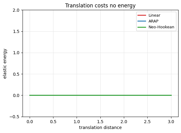
Sliding the triangle leaves every energy flat at zero. (We fix the y-axis so the flat line doesn’t look like noise.)
d = np.linspace(0, 3, 40)
states = [translate(X, [dx, 0.0]) for dx in d]
series = {name: np.zeros_like(d) for name in ENERGIES}
for i, U in enumerate(states):
    F = simkit.deformation_gradient(X, T, U)[0]
    for name, fn in ENERGIES.items():
        series[name][i] = fn(F)

utils.line_plot(d, series, xlabel="translation distance", ylabel="elastic energy",
                title="Translation costs no energy", ylim=(-0.5, 2.0))
plt.show()

fig, anim = utils.animate_scene_energy(states, d, series, rest=X,
    xlabel="translation distance", lims=((-1.2, 4.0), (-1.2, 1.6)),
    scene_title="triangle sliding", title="energy vs translation", fps=20,
    energy_ylim=(-0.5, 2.0))      # fixed y-axis (matches the static plot) -> flat line
utils.show_video(fig, anim, "media/03_translation.mp4", fps=20)
Scale: every energy grows (the intuitive case)#
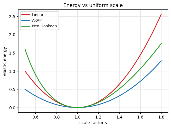
Uniform scaling genuinely deforms the material, so all three energies rise as we move away from \(s = 1\).
s = np.linspace(0.5, 1.8, 50)
states = [scale(X, si) for si in s]
series = {name: np.zeros_like(s) for name in ENERGIES}
for i, U in enumerate(states):
    F = simkit.deformation_gradient(X, T, U)[0]
    for name, fn in ENERGIES.items():
        series[name][i] = fn(F)

utils.line_plot(s, series, xlabel="scale factor s", ylabel="elastic energy",
                title="Energy vs uniform scale")
plt.show()
fig, anim = utils.animate_scene_energy(states, s, series, rest=X, xlabel="scale factor s",
    scene_title="triangle scaling", title="energy vs scale", fps=20)
utils.show_video(fig, anim, "media/03_scale.mp4", fps=20)
Shear: every energy grows too#
k = np.linspace(0.0, 1.6, 50)
states = [shear(X, ki) for ki in k]
series = {name: np.zeros_like(k) for name in ENERGIES}
for i, U in enumerate(states):
    F = simkit.deformation_gradient(X, T, U)[0]
    for name, fn in ENERGIES.items():
        series[name][i] = fn(F)

utils.line_plot(k, series, xlabel="shear k", ylabel="elastic energy",
                title="Energy vs shear")
plt.show()
fig, anim = utils.animate_scene_energy(states, k, series, rest=X, xlabel="shear k",
    scene_title="triangle shearing", title="energy vs shear", fps=20)
utils.show_video(fig, anim, "media/03_shear.mp4", fps=20)
Rotation: linear elasticity is not rotation-invariant#
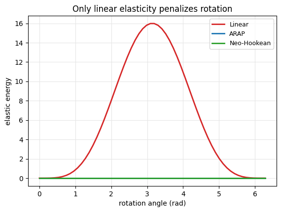
Now the surprise. Spin the triangle through a full turn. ARAP and Neo-Hookean stay at zero — rotation is free. Linear elasticity rises and falls: its small-strain tensor \(\varepsilon\) mistakes rotation for stretch. This is why linear elasticity is only valid for tiny deformations.
ang = np.linspace(0, 2 * np.pi, 60)
states = [rotate(X, a) for a in ang]
series = {name: np.zeros_like(ang) for name in ENERGIES}
for i, U in enumerate(states):
    F = simkit.deformation_gradient(X, T, U)[0]
    for name, fn in ENERGIES.items():
        series[name][i] = fn(F)

utils.line_plot(ang, series, xlabel="rotation angle (rad)", ylabel="elastic energy",
                title="Only linear elasticity penalizes rotation")
plt.show()
fig, anim = utils.animate_scene_energy(states, ang, series, rest=X,
    xlabel="rotation angle (rad)", scene_title="triangle rotating",
    title="energy vs rotation angle", fps=20)
utils.show_video(fig, anim, "media/03_rotation.mp4", fps=20)
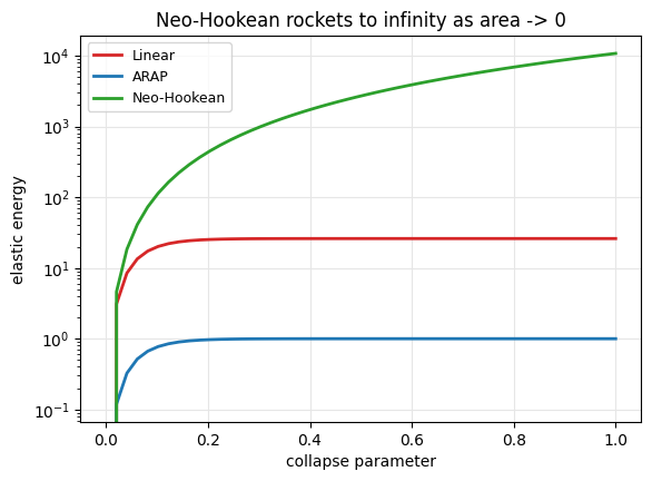
Crushing the triangle flat: Neo-Hookean \(\to \infty\)#
Drive the apex down toward the base so the area \(J = \det F \to 0\).
Why didn’t it explode before? The Neo-Hookean blow-up is real but only logarithmic: \(\psi \approx \tfrac{\lambda}{2}(\ln J)^2 - \mu\ln J\). Since \(\ln J\) grows slowly, you have to (a) drive \(J\) extremely close to zero and (b) use a stiff, nearly-incompressible material (large \(\lambda\)) for the number to actually rocket. So here we collapse hard — \(y = y_0\,10^{-9t}\), i.e. \(J\) down to \(\sim 10^{-9}\) — with \(\lambda = 50\). Now Neo-Hookean reaches \(\sim 10^4\) and is climbing to \(+\infty\), while ARAP sits at a finite plateau (it has no volume term) and linear stays modest. We plot on a log axis.
t = np.linspace(0, 1, 50)
y0 = X[2, 1]
def collapse_apex(frac):
    U = X.copy(); U[2, 1] = y0 * 10.0**(-9.0 * frac); return U   # hard log collapse -> J ~ 1e-9
states = [collapse_apex(f) for f in t]
series = {name: np.zeros_like(t) for name in ENERGIES}
for i, U in enumerate(states):
    F = simkit.deformation_gradient(X, T, U)[0]
    for name, fn in ENERGIES.items():
        series[name][i] = fn(F, mu=1.0, lam=50.0)               # nearly-incompressible: lam >> mu

Jend = np.linalg.det(simkit.deformation_gradient(X, T, states[-1])[0])
print(f"det F at full collapse: {Jend:.2e}   Neo-Hookean energy: {series['Neo-Hookean'][-1]:.0f}")

utils.line_plot(t, series, xlabel="collapse parameter", ylabel="elastic energy",
                logy=True, title="Neo-Hookean rockets to infinity as area -> 0")
plt.show()
fig, anim = utils.animate_scene_energy(states, t, series, rest=X,
    xlabel="collapse parameter", scene_title="apex crushed onto the base",
    title="energy vs collapse", logy=True, fps=18)
utils.show_video(fig, anim, "media/03_collapse.mp4", fps=18)
det F at full collapse: 1.00e-09 Neo-Hookean energy: 10757
Takeaways#
We wrote each energy in one line: linear (strain tensor), ARAP (distance to a rotation), Neo-Hookean (with the \(-\mu\ln J\) inversion barrier).
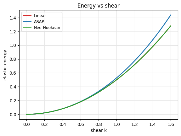
Good energies are zero for rigid motion and grow with scale/shear.
Linear breaks rotation-invariance; Neo-Hookean diverges at collapse; ARAP saturates.
Next: minimize an energy (plus constraints) to actually pose a shape.