10 · Resolution and Cost: the Accuracy/Speed Trade-off#
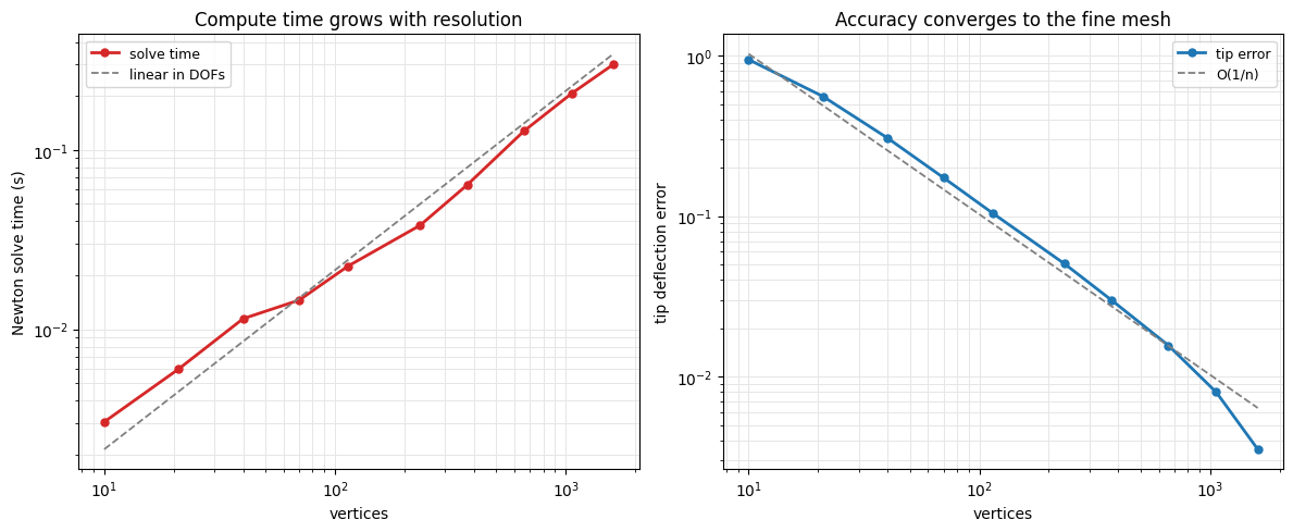
Refining the mesh improves accuracy but makes every solve more expensive. We measure both on a cantilever sagging under gravity:
cost: Newton-solve time vs. vertex count (10 resolutions),
accuracy: tip deflection converging to a very fine reference,
the punchline: a super-fine mesh is accurate but too slow to iterate on.
%matplotlib inline
import time
import numpy as np
import scipy as sp
import matplotlib.pyplot as plt
import simkit
from simkit.solvers import newton_solver
import utils
A timed static solve at any resolution#
GravityBeam is our standard static simulator: it builds the mesh, precomputes
the per-mesh constants once, and composes three energy terms — the elastic
material, a fixed pin on the left edge, and gravity — summing them
one per line. The beam is soft enough (\(E = 800\)) that the sag is large and
obvious. gravity_scale lets us ramp gravity for the animation, and .solve()
returns the settled equilibrium.
class GravityBeam:
    """Cantilever sagging under gravity: elastic + pin + gravity, solved with Newton."""

    def __init__(self, nx, ny):
        X, T = utils.triangulated_grid(nx, ny, width=2.0, height=0.3)
        self.X, self.T = X, T
        self.p   = utils.precompute(X, T, ym=800.0, pr=0.4, rho=1.0, gravity=-9.8)
        self.psi = utils.make_material("Neo-Hookean")
        pin_idx  = np.where(X[:, 0] <= X[:, 0].min() + 1e-6)[0]
        self.pin = utils.PenaltySpring(self.p.n, self.p.dim, 1e7).set(pin_idx, X[pin_idx])
        self.gravity = utils.Gravity(self.p.f_g)

    def energy(self, x):
        E_elastic = self.psi.energy(x, self.p)
        E_pin     = self.pin.energy(x)
        E_gravity = self.gravity.energy(x)
        return E_elastic + E_pin + E_gravity

    def gradient(self, x):
        g_elastic = self.psi.gradient(x, self.p)
        g_pin     = self.pin.gradient(x)
        g_gravity = self.gravity.gradient(x)
        return g_elastic + g_pin + g_gravity

    def hessian(self, x):
        H_elastic = self.psi.hessian(x, self.p)
        H_pin     = self.pin.hessian(x)
        return H_elastic + H_pin

    def solve(self, iters=30):
        x = newton_solver(self.X.reshape(-1, 1), self.energy, self.gradient, self.hessian,
                          max_iter=iters, do_line_search=True)
        return x.reshape(self.p.n, self.p.dim)
Cost and accuracy across 10 resolutions#
We loop explicitly over ten resolutions: build a GravityBeam, time its
.solve() with time.perf_counter, and record the vertex count, solve time,
and tip deflection (the \(y\) of the right-most vertex). A very fine mesh serves
as the “ground truth” tip deflection, and the error of each run is its tip
deflection’s distance from that reference.
resolutions = [(5, 2), (7, 3), (10, 4), (14, 5), (19, 6), (26, 9), (34, 11), (44, 15), (56, 19), (70, 23)]

verts, times, tips = [], [], []
for nx, ny in resolutions:
    beam = GravityBeam(nx, ny)
    t0 = time.perf_counter()
    U = beam.solve()
    dt = time.perf_counter() - t0
    verts.append(beam.p.n)
    times.append(dt)
    tips.append(U[int(np.argmax(beam.X[:, 0])), 1])

ref_beam = GravityBeam(90, 30)                       # fine "ground truth"
t0 = time.perf_counter()
ref_U = ref_beam.solve()
ref_time = time.perf_counter() - t0
ref_tip  = ref_U[int(np.argmax(ref_beam.X[:, 0])), 1]
print(f"fine reference: {ref_beam.p.n} verts, {ref_time*1000:.0f} ms, tip_y = {ref_tip:.4f}")

verts  = np.array(verts)
times  = np.array(times)
errors = np.array([abs(t - ref_tip) for t in tips])
for n, dt, ty, e in zip(verts, times, tips, errors):
    print(f"  {n:5d} verts   {dt*1000:7.1f} ms   tip_y {ty:.4f}   error {e:.2e}")
fine reference: 2700 verts, 639 ms, tip_y = -1.5929
     10 verts       3.0 ms   tip_y -0.6471   error 9.46e-01
     21 verts       6.0 ms   tip_y -1.0354   error 5.57e-01
     40 verts      11.4 ms   tip_y -1.2861   error 3.07e-01
     70 verts      14.5 ms   tip_y -1.4194   error 1.73e-01
    114 verts      22.5 ms   tip_y -1.4883   error 1.05e-01
    234 verts      38.0 ms   tip_y -1.5424   error 5.05e-02
    374 verts      63.8 ms   tip_y -1.5629   error 3.00e-02
    660 verts     127.8 ms   tip_y -1.5772   error 1.56e-02
   1064 verts     207.3 ms   tip_y -1.5849   error 8.00e-03
   1610 verts     300.5 ms   tip_y -1.5894   error 3.52e-03
Compute time vs resolution, and accuracy vs resolution#
fig, axes = plt.subplots(1, 2, figsize=(12, 5))
utils.loglog_plot(verts, {"solve time": times}, xlabel="vertices", ylabel="Newton solve time (s)",
    colors={"solve time": "#d62728"}, ref_slopes={"linear in DOFs": 1},
    title="Compute time grows with resolution", markers=True, ax=axes[0])
utils.loglog_plot(verts, {"tip error": errors}, xlabel="vertices", ylabel="tip deflection error",
    colors={"tip error": "#1f77b4"}, ref_slopes={"O(1/n)": -1},
    title="Accuracy converges to the fine mesh", markers=True, ax=axes[1])
fig.tight_layout(); plt.show()
Watching three resolutions sag (clearly!) under gravity#
Ramp gravity \(0 \rightarrow 1\) and solve each frame for three resolutions, then hold at full gravity so every beam settles to its final equilibrium and visibly comes to rest. They converge to nearly the same big droop — but the finest one took far longer per frame.
ramp = np.concatenate([np.linspace(0.0, 1.0, 22), np.ones(12)])   # ramp up, then hold at rest
panels = []
for nx, ny, label in [(7, 3, "coarse"), (16, 6, "medium"), (32, 11, "fine")]:
    beam = GravityBeam(nx, ny)
    f_g_full = beam.p.f_g.copy()                                  # scale gravity for the ramp
    states = []
    for g in ramp:
        beam.gravity.f_g = g * f_g_full
        states.append(beam.solve())
    panels.append({"states": states, "T": beam.T,
                   "title": f"{label}  ({beam.p.n} verts)"})

fig, anim = utils.animate_meshes_grid(panels, lims=((-1.2, 1.2), (-1.8, 0.3)), fps=20,
    suptitle="Same beam, three resolutions, sagging under gravity")
utils.show_video(fig, anim, "media/10_resolution.mp4", fps=20)
Why “just refine it” is a trap#
i_good = 4                                            # a mid-resolution mesh
rel = errors[i_good] / abs(ref_tip)
print(f"good-enough ({verts[i_good]:5d} verts): {times[i_good]*1000:8.1f} ms/solve   ({rel*100:.0f}% tip error)")
print(f"fine        ({ref_beam.p.n:5d} verts): {ref_time*1000:8.1f} ms/solve")
print(f"\nThe fine mesh is ~{ref_time/times[i_good]:.0f}x slower per solve for a tip deflection")
print(f"within {rel*100:.0f}% of it. Interactive editing (many solves/second) is impossible")
print("long before that accuracy is worth it -- pick the coarsest mesh that captures the behavior.")
good-enough (  114 verts):     22.5 ms/solve   (7% tip error)
fine        ( 2700 verts):    638.8 ms/solve

The fine mesh is ~28x slower per solve for a tip deflection
within 7% of it. Interactive editing (many solves/second) is impossible
long before that accuracy is worth it -- pick the coarsest mesh that captures the behavior.
Takeaways#
Cost rises steeply with vertex count; each Newton step solves a bigger sparse system.
Accuracy improves with resolution but with diminishing returns.
A super-fine mesh is accurate yet too slow to iterate on.
That completes the offline SimKit tutorial series (1–10): building and understanding the deformation gradient, elastic energies, the elastostatic minimization, the solvers and line search that drive it, time integration, contact, and the resolution/cost trade-off.