13 · Outline Areas: the shoelace formula, its gradient, and its Hessian

A closed outline (or chamber) is a loop of edges through a shared set of 2D vertices. simkit measures the signed area each loop encloses with outline_areas, and provides its first and second derivatives with outline_areas_gradient and outline_areas_hessian. This notebook walks through all three, top to bottom:

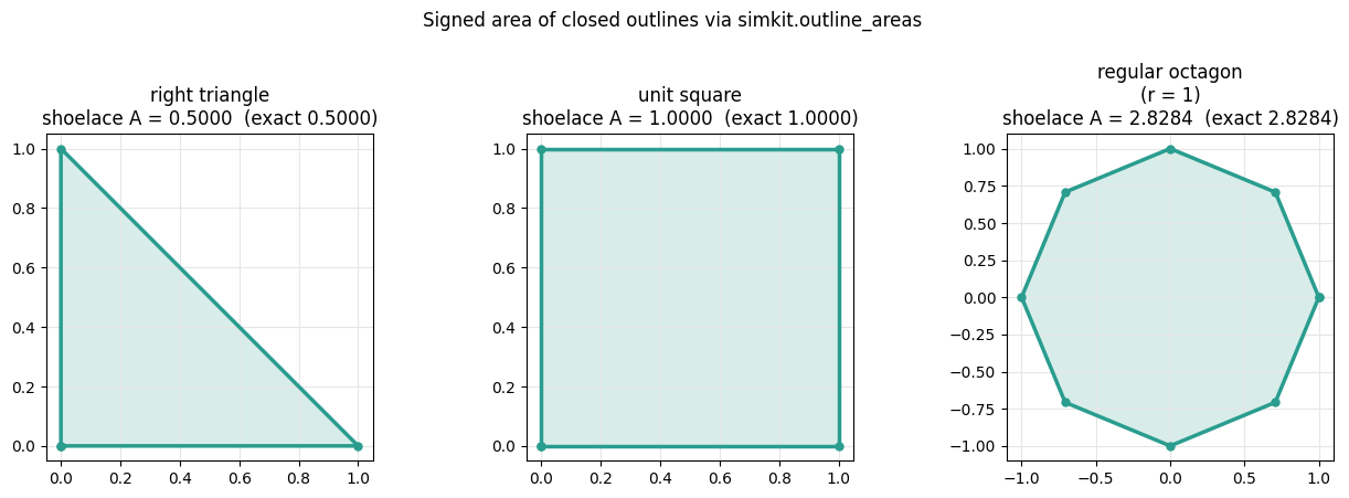
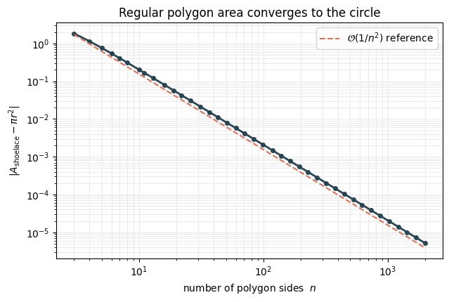
1. Known areas. Measure a triangle, a square, and a regular polygon, and watch the polygon’s area converge to \(\pi r^2\) as it gains sides.

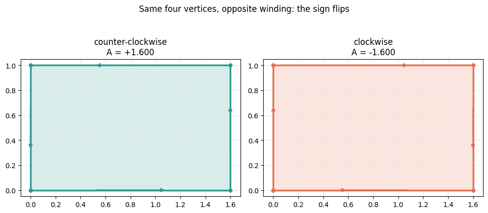
2. Orientation = sign. Walk the same loop clockwise vs counter-clockwise and watch the sign flip. This is why simkit keeps the signed area: it is a smooth polynomial of the vertices, differentiable everywhere.

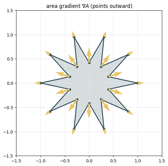
3. The gradient inflates the shape. \(\nabla A\) is the direction each vertex should move to grow the area; it points along the outward normal. We draw that field, then follow it to inflate a star while the area climbs monotonically.

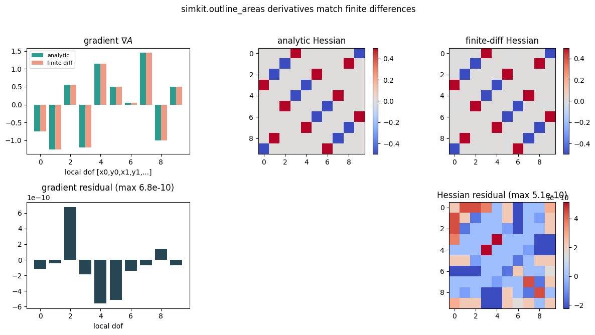
4. Checking the derivatives. The analytic gradient and (constant) Hessian are compared against finite differences, the same checks the unit tests make.

%matplotlib inline
import numpy as np
import matplotlib.pyplot as plt
from matplotlib.animation import FuncAnimation

import simkit
import utils

# A small consistent palette.
POS_C = "#2a9d8f"   # positive / CCW area
NEG_C = "#e76f51"   # negative / CW area
EDGE_C = "#264653"
GRAD_C = "#e9c46a"


def regular_polygon(n, r=1.0, center=(0.0, 0.0)):
    # n vertices spaced counter-clockwise on a circle of radius r.
    theta = np.linspace(0.0, 2.0 * np.pi, n, endpoint=False)
    return np.column_stack([center[0] + r * np.cos(theta),
                            center[1] + r * np.sin(theta)])


def draw_outline(ax, X, color, fill=True, lw=2.5):
    # Draw a closed outline (and optionally fill it) on ax.
    loop = np.vstack([X, X[0]])
    if fill:
        ax.fill(X[:, 0], X[:, 1], color=color, alpha=0.18, zorder=1)
    ax.plot(loop[:, 0], loop[:, 1], "-o", color=color, lw=lw, ms=5, zorder=3)

1 · Known areas: the shoelace formula on shapes we can check by hand

For a closed loop of vertices the signed area is the shoelace (Gauss) formula

\[ A = \tfrac{1}{2} \sum_{(i,j)\in E} \big(x_i\, y_j - x_j\, y_i\big). \]

Each term is twice the signed area of the triangle (origin, \(p_i\), \(p_j\)); summing around the loop, the parts outside the polygon cancel and only the enclosed area survives. We test it on three shapes whose area we already know:

• right triangle with legs 1  →  \(A = \tfrac12\)

• unit square  →  \(A = 1\)

• regular \(n\)-gon of radius \(r\)  →  \(A = \tfrac12 n r^2 \sin(2\pi/n)\)

That last one is the nicest: a regular polygon is just a circle we have not finished drawing, so its shoelace area marches up to \(\pi r^2\) as \(n\) grows.

shapes = [
    ("right triangle", np.array([[0.0, 0.0], [1.0, 0.0], [0.0, 1.0]]), 0.5),
    ("unit square", np.array([[0.0, 0.0], [1.0, 0.0], [1.0, 1.0], [0.0, 1.0]]), 1.0),
    ("regular octagon\n(r = 1)", regular_polygon(8, r=1.0),
     0.5 * 8 * 1.0 ** 2 * np.sin(2 * np.pi / 8)),
]

fig, axes = plt.subplots(1, 3, figsize=(13, 4.2))
for ax, (name, X, exact) in zip(axes, shapes):
    E = simkit.closed_polyline(X)
    A = simkit.outline_areas(X, [E])[0]
    draw_outline(ax, X, POS_C)
    utils.setup_axes(ax, title=f"{name}\nshoelace A = {A:.4f}  (exact {exact:.4f})")
fig.suptitle("Signed area of closed outlines via simkit.outline_areas", y=1.03)
fig.tight_layout()
fig.savefig("media/13_known_areas.png", dpi=130, bbox_inches="tight")
plt.show()

# Convergence of the regular n-gon area to the circle pi r^2.
r = 1.0
ns = np.unique(np.round(np.logspace(np.log10(3), np.log10(2000), 40)).astype(int))
err = []
for n in ns:
    Xn = regular_polygon(int(n), r=r)
    En = simkit.closed_polyline(Xn)
    A = simkit.outline_areas(Xn, [En])[0]
    err.append(abs(A - np.pi * r ** 2))

fig, ax = plt.subplots(figsize=(6.5, 4.4))
ax.loglog(ns, err, "-o", color=EDGE_C, ms=4, lw=2)
ax.loglog(ns, 0.5 * np.pi ** 3 / ns ** 2, "--", color=NEG_C, lw=1.5,
          label=r"$\mathcal{O}(1/n^2)$ reference")
ax.set_xlabel("number of polygon sides  $n$")
ax.set_ylabel(r"$|A_{\mathrm{shoelace}} - \pi r^2|$")
ax.set_title("Regular polygon area converges to the circle")
ax.grid(True, which="both", color="0.92")
ax.legend()
fig.tight_layout()
fig.savefig("media/13_circle_convergence.png", dpi=130, bbox_inches="tight")
plt.show()

2 · Orientation is the sign of the area

The shoelace area is signed: traverse a loop counter-clockwise and you get a positive number, traverse the exact same loop clockwise and you get its negative. simkit deliberately keeps this sign instead of taking \(|A|\), because the signed area is a smooth polynomial in the vertex coordinates — so its gradient and Hessian (sections 3-4) are exact everywhere, including the degenerate \(A = 0\) case where \(|A|\) has a non-differentiable kink.

X = np.array([[0.0, 0.0], [1.6, 0.0], [1.6, 1.0], [0.0, 1.0]])
E_ccw = simkit.closed_polyline(X)
E_cw = E_ccw[::-1, ::-1]                 # same loop, walked the other way

A_ccw = simkit.outline_areas(X, [E_ccw])[0]
A_cw = simkit.outline_areas(X, [E_cw])[0]
print(f"counter-clockwise A = {A_ccw:+.3f},  clockwise A = {A_cw:+.3f}")

fig, axes = plt.subplots(1, 2, figsize=(10, 4.4))
for ax, (E, A, c, label) in zip(
    axes,
    [(E_ccw, A_ccw, POS_C, "counter-clockwise"),
     (E_cw, A_cw, NEG_C, "clockwise")],
):
    draw_outline(ax, X, c)
    for a, b in E:                       # arrowheads showing the winding direction
        mid = 0.5 * (X[a] + X[b])
        d = X[b] - X[a]
        ax.annotate("", xy=mid + 0.18 * d, xytext=mid - 0.18 * d,
                    arrowprops=dict(arrowstyle="-|>", color=c, lw=2))
    utils.setup_axes(ax, title=f"{label}\nA = {A:+.3f}")
fig.suptitle("Same four vertices, opposite winding: the sign flips", y=1.03)
fig.tight_layout()
fig.savefig("media/13_orientation_sign.png", dpi=130, bbox_inches="tight")
plt.show()

counter-clockwise A = +1.600,  clockwise A = -1.600

3 · The gradient inflates the shape

outline_areas_gradient returns \(\partial A/\partial x\) for every vertex of the loop, stacked as [dx0, dy0, dx1, dy1, ...]. Geometrically

\[ \frac{\partial A}{\partial x_i} = \tfrac12 (y_{i+1} - y_{i-1}), \qquad \frac{\partial A}{\partial y_i} = -\tfrac12 (x_{i+1} - x_{i-1}), \]

so the area grows fastest when vertex \(i\) moves along its outward normal, by an amount proportional to the length of its two incident edges. The gradient field is therefore a ring of outward arrows.

Follow that field — \(x \leftarrow x + \mathrm{d}t\,\nabla A\) — and the loop inflates: every step is guaranteed to increase the area because we move straight uphill on \(A\). We start from a spiky star so the inflation is dramatic.

# A 10-point star: alternate far / near radii.
n_arms = 10
ang = np.linspace(0.0, 2.0 * np.pi, 2 * n_arms, endpoint=False)
rad = np.where(np.arange(2 * n_arms) % 2 == 0, 1.0, 0.42)
X0 = np.column_stack([rad * np.cos(ang), rad * np.sin(ang)])
E = simkit.closed_polyline(X0)

# Per-vertex area gradient reshaped to (n, 2) in this loop's vertex order.
g = simkit.outline_areas_gradient(X0, [E])[0].reshape(-1, 2)

fig, ax = plt.subplots(figsize=(5.6, 5.6))
draw_outline(ax, X0, EDGE_C, fill=True, lw=2)
ax.quiver(X0[:, 0], X0[:, 1], g[:, 0], g[:, 1],
          color=GRAD_C, angles="xy", scale_units="xy", scale=1.0,
          width=0.012, zorder=5)
utils.setup_axes(ax, (-1.5, 1.5), (-1.5, 1.5),
                 title="area gradient $\\nabla A$ (points outward)")
fig.tight_layout()
fig.savefig("media/13_gradient_field.png", dpi=130, bbox_inches="tight")
plt.show()

# Gradient ascent: inflate the star, recording the area at every step.
dt, n_steps = 0.08, 90
states = [X0.copy()]
areas = [simkit.outline_areas(X0, [E])[0]]
X = X0.copy()
for _ in range(n_steps):
    g = simkit.outline_areas_gradient(X, [E])[0].reshape(-1, 2)
    X = X + dt * g                       # one step straight uphill on A
    states.append(X.copy())
    areas.append(simkit.outline_areas(X, [E])[0])
print(f"area grew from {areas[0]:.3f} to {areas[-1]:.3f} "
      f"(monotone: {np.all(np.diff(areas) > 0)})")

area grew from 1.298 to 126.337 (monotone: True)

# Animate the inflation with the area curve filling in beside it.
fig, (ax_s, ax_a) = plt.subplots(1, 2, figsize=(11, 5))
lim = 1.05 * np.max(np.abs(states[-1]))
utils.setup_axes(ax_s, (-lim, lim), (-lim, lim), title="inflating the star")
(loop_line,) = ax_s.plot([], [], "-o", color=POS_C, lw=2.5, ms=4)
fill_holder = {"p": None}

ax_a.set_xlim(0, n_steps)
ax_a.set_ylim(areas[0] * 0.9, areas[-1] * 1.05)
ax_a.set_xlabel("gradient-ascent step")
ax_a.set_ylabel("enclosed area  $A$")
ax_a.set_title("area climbs every step")
ax_a.grid(True, color="0.92")
(area_line,) = ax_a.plot([], [], color=POS_C, lw=2.5)

def update(k):
    Xk = states[k]
    loop = np.vstack([Xk, Xk[0]])
    loop_line.set_data(loop[:, 0], loop[:, 1])
    if fill_holder["p"] is not None:
        fill_holder["p"].remove()
    fill_holder["p"] = ax_s.fill(Xk[:, 0], Xk[:, 1], color=POS_C, alpha=0.18, zorder=1)[0]
    area_line.set_data(np.arange(k + 1), areas[:k + 1])
    return loop_line, area_line

anim = FuncAnimation(fig, update, frames=len(states), interval=50, blit=False)
fig.suptitle("Following $\\nabla A$ inflates the loop and grows its area", y=1.0)
fig.tight_layout()
utils.show_video(fig, anim, "media/13_inflate.mp4", fps=20)

4 · Checking the gradient and Hessian against finite differences

The analytic derivatives should match a brute-force central finite difference of outline_areas. We show that as heatmaps: analytic vs FD, plus the tiny residual. The Hessian is especially clean — the signed area is bilinear in the coordinates, so \(\partial^2 A/\partial x^2\) is a constant matrix that only couples the \(x\) of one endpoint to the \(y\) of the other (the checkerboard pattern below), and it does not depend on where the vertices are at all.

X = np.array([[0.0, 0.0], [2.0, -0.3], [2.4, 1.1],
              [1.0, 2.0], [-0.5, 1.2]])          # irregular pentagon
E = simkit.closed_polyline(X)
z = X.flatten()

def area_flat(zz):                                # all verts in one loop ->
    return simkit.outline_areas(zz.reshape(-1, 2), [E])   # local dofs == X.flatten()

g = simkit.outline_areas_gradient(X, [E])[0].flatten()
g_fd = simkit.gradient_cfd(area_flat, z, 1e-6).flatten()
H = simkit.outline_areas_hessian(X, [E])[0]
H_fd = simkit.hessian_cfd(area_flat, z, 1e-3).reshape(H.shape)
print(f"max |grad - fd| = {np.max(np.abs(g - g_fd)):.2e}")
print(f"max |Hess - fd| = {np.max(np.abs(H - H_fd)):.2e}")

fig = plt.figure(figsize=(12, 6.5))
ax_g = fig.add_subplot(2, 3, 1)
idx = np.arange(len(g))
ax_g.bar(idx - 0.2, g, width=0.4, color=POS_C, label="analytic")
ax_g.bar(idx + 0.2, g_fd, width=0.4, color=NEG_C, alpha=0.7, label="finite diff")
ax_g.set_title("gradient $\\nabla A$"); ax_g.set_xlabel("local dof [x0,y0,x1,y1,...]")
ax_g.legend(fontsize=8)

ax_gr = fig.add_subplot(2, 3, 4)
ax_gr.bar(idx, g - g_fd, color=EDGE_C)
ax_gr.set_title(f"gradient residual (max {np.max(np.abs(g-g_fd)):.1e})")
ax_gr.set_xlabel("local dof")

vmax = max(np.max(np.abs(H)), 1e-9)
for col, (M, title) in enumerate([(H, "analytic Hessian"), (H_fd, "finite-diff Hessian")]):
    ax = fig.add_subplot(2, 3, 2 + col)
    im = ax.imshow(M, cmap="coolwarm", vmin=-vmax, vmax=vmax)
    ax.set_title(title); fig.colorbar(im, ax=ax, fraction=0.046)
ax_hr = fig.add_subplot(2, 3, 6)
im = ax_hr.imshow(H - H_fd, cmap="coolwarm")
ax_hr.set_title(f"Hessian residual (max {np.max(np.abs(H-H_fd)):.1e})")
fig.colorbar(im, ax=ax_hr, fraction=0.046)

fig.suptitle("simkit.outline_areas derivatives match finite differences", y=1.02)
fig.tight_layout()
fig.savefig("media/13_derivative_checks.png", dpi=130, bbox_inches="tight")
plt.show()

max |grad - fd| = 6.78e-10
max |Hess - fd| = 5.14e-10