23 · Fast Complementary Dynamics — secondary motion that never fights the rig#
An animator poses a character with a rig: a few handles driving a smooth Linear Blend Skinning (LBS) deformation. Complementary dynamics (Zhang et al. 2020) layers physical secondary motion — jiggle, sag, follow-through — on top of that rig, under one rule: the simulation may never reproduce a motion the rig can already make itself.
Split every vertex’s displacement into a rig part and a complementary part,
and constrain the complementary part to be orthogonal to the rig:
\(J\) — the LBS Jacobian of the rig. Its columns span every displacement the handles can produce, i.e. the control space.
\(M\) — the mass matrix, so “orthogonal” is measured in the physical momentum inner product: \(u_c\) carries no momentum that the rig already accounts for.
\(D\) — a diagonal momentum-leaking field. Where \(D=1\) momentum is conserved against the rig; where \(D\to 0\) momentum is allowed to leak, letting that tissue ride along with the handle instead of resisting it.
We build this twice. First a full-order solver, to watch the constraint do its job. Then the
fast version of Fast Complementary Dynamics via Skinning Eigenmodes (Benchekroun et al.,
SIGGRAPH 2023), which makes it real-time with two simkit ingredients: rig-orthogonal skinning
eigenmodes and rotation clustering.
%matplotlib inline
import time, warnings
import numpy as np
import scipy as sp
import scipy.sparse as sps
import igl
import matplotlib.pyplot as plt
from matplotlib.animation import FuncAnimation
import utils
from simkit import (massmatrix, deformation_jacobian, lbs_jacobian, volume,
                    ympr_to_lame, polar_svd, orthonormalize,
                    project_into_subspace, cluster_grouping_matrices)
from simkit.diffuse_field import diffuse_field
from simkit.normalize_and_center import normalize_and_center
from simkit.lbs_weight_space_constraint import lbs_weight_space_constraint
from simkit.skinning_eigenmodes import skinning_eigenmodes
from simkit.spectral_cubature import spectral_cubature
from simkit.solvers import block_coord
warnings.filterwarnings("ignore"); np.seterr(all="ignore")

YM, RHO, DT = 1e5, 1e3, 1e-2          # Young's modulus, density, timestep
RIG_C, FULL_C, RED_C = "#d62728", "#1f77b4", "#2ca02c"   # rig / full / reduced colors
1 · The rig: one global handle#
The simplest possible rig is a single affine handle — one LBS bone with weight \(1\)
everywhere. lbs_jacobian(X, ones) builds its Jacobian \(J\), whose \(6\) columns (in 2D) span
every affine map: translation, rotation, scale, shear. The animator’s pose is a vector of rig
parameters \(p\), and the rigged shape is simply \(x = J\,p\).
Here the animation is a metronome: sweep the handle’s \(x\)-translation left and right. On its own the beam stays perfectly rigid — there is no physics yet.
X, T = beam(); n, dim = X.shape
op = elastic_operators(X, T)
J  = lbs_jacobian(X, np.ones((n, 1)))          # control space: one global affine handle
p0 = rig_rest(J, op["Mv"], X)
print(f"mesh: {n} verts, {T.shape[0]} triangles   |   rig: J is {J.shape} -> {J.shape[1]} DOFs")

NSTEPS = 200
rig_states = [(J @ handle(p0, i)).reshape(n, dim) for i in range(NSTEPS)]

fig, anim = animate_panels(
    [dict(states=thin(rig_states), T=T, title="rig pose  $x = J\\,p$", color=RIG_C)],
    suptitle="The animator's input: a rigid beam swept left and right")
utils.show_video(fig, anim, "media/23_rig.mp4", fps=30)
mesh: 200 verts, 312 triangles | rig: J is (400, 6) -> 6 DOFs
2 · Full-order complementary dynamics#
Now add physics. Each timestep is a backward-Euler implicit step that minimizes the usual inertia-plus-elasticity objective over the total position \(x = J\,p_{\text{next}} + u_c\),
where \(y = x_{\text{curr}} + h\,\dot x\) is the inertial prediction. The only thing that makes this complementary dynamics rather than ordinary elastodynamics is that one linear constraint.
We solve the ARAP minimization with block coordinate descent (tutorials 21 & 22):
local step — for each triangle, the closest rotation to its current deformation gradient (one
polar_svdper element);global step — a single linear solve for \(u_c\). With the constraint, that solve becomes a KKT system \(\begin{bmatrix} H & A^{\top}\\ A & 0\end{bmatrix}\) with \(A = J^{\top} M D\). Both \(H = L + M/h^2\) and \(A\) are constant, so we prefactor once and reuse the factorization every step and every inner iteration.
The momentum-leaking field \(D\) is built by diffusing a value of \(1\) inward from the boundary
(diffuse_field) and using \(1-\text{(that)}\): near the handle/boundary momentum leaks (tissue
follows the rig), deep inside it is conserved (tissue resists, producing secondary motion).
FullCD does all of this precompute in __init__ and exposes a step(...) method.
class FullCD:
    """Full-order complementary dynamics: per-element rotations + a prefactored
    KKT global step enforcing the rig-orthogonality constraint  J^T M D u_c = 0."""

    def __init__(self, X, T):
        n, dim = X.shape
        op = elastic_operators(X, T)
        self.Mv, self.G, self.AMue, self.L = op["Mv"], op["G"], op["AMue"], op["L"]
        self.dim = dim

        # rig J: one global affine handle, and the rest pose that matches X
        self.J  = lbs_jacobian(X, np.ones((n, 1)))
        self.p0 = rig_rest(self.J, self.Mv, X)

        # momentum-leaking field D: ~0 near the boundary (leaks), ->1 in the interior (conserved)
        bnd  = np.unique(igl.boundary_facets(T)[0])
        leak = diffuse_field(X, T, bnd, np.ones((bnd.shape[0], 1)), dt=1, normalize=True)
        D    = sps.kron(sps.diags((1 - leak).flatten()), sps.identity(dim))

        # rig-orthogonality operator A = J^T M D, and the constant backward-Euler matrix H
        self.A = sps.csc_matrix(self.J.T @ self.Mv @ D)
        self.H = (self.L + self.Mv / DT**2).tocsc()

        # prefactor the KKT system [[H, A^T], [A, 0]] once, reuse every step / inner iter
        KKT = sps.bmat([[self.H, self.A.T],
                        [self.A, sps.csc_matrix((self.A.shape[0],) * 2)]]).tocsc()
        self.kkt = sps.linalg.factorized(KKT)
        self.nc  = self.A.shape[0]

        self.state_dim = n * dim
        self.n_rot     = T.shape[0]
        self.B         = None        # full order: u_c lives in full coordinates

    def step(self, uc, uc_dot, p, p_dot, p_next, iters=10):
        Jp = self.J @ p_next
        y  = (uc + DT * uc_dot) + self.J @ (p + DT * p_dot)      # inertial prediction

        def local(u):                                            # closest rotation, per triangle
            return polar_svd((self.G @ (Jp + u)).reshape(-1, self.dim, self.dim))[0].reshape(-1, 1)

        def glob(u, R):                                          # constrained (rig-orthogonal) solve
            E_inertia = self.Mv @ y / DT**2                      # backward-Euler inertia term
            E_elastic = self.G.T @ (self.AMue @ R)               # ARAP (local-rotation) elastic term
            E_rigpose = -self.H @ Jp                             # pin the rig pose into the rhs
            rhs = E_inertia + E_elastic + E_rigpose
            return self.kkt(np.vstack([rhs, np.zeros((self.nc, 1))]))[:uc.shape[0]]

        return block_coord(uc.copy(), glob, local, 0.0, iters)
Rolling out a solver under the metronome rig#
The roll-out is the same for both solvers: at each step, advance the handle pose, take one implicit step for the complementary state, finite-difference the velocities, and record both the deformed mesh and the rig-orthogonality residual \(\lVert J^{\top} M D\,u_c\rVert\). For the reduced solver the state lives in subspace coordinates \(z\), so we lift \(u_c = B\,z\) before measuring.
def run(solver, nsteps=NSTEPS):
    """Roll out a solver under the left/right handle sweep. Returns (states, violation)."""
    J, p0, B = solver.J, solver.p0, solver.B
    s = np.zeros((solver.state_dim, 1)); s_dot = np.zeros_like(s)
    p = p0.copy(); p_dot = np.zeros_like(p)
    states, viol = [], []
    for i in range(nsteps):
        p_next = handle(p0, i)
        s_new  = solver.step(s, s_dot, p, p_dot, p_next)
        s_dot  = (s_new - s) / DT; p_dot = (p_next - p) / DT
        s, p   = s_new, p_next.copy()
        uc = (B @ s) if B is not None else s                # u_c in full coordinates
        states.append((J @ p + uc).reshape(-1, dim))
        viol.append(float(np.linalg.norm(solver.A @ uc)))
    return states, viol

full = FullCD(X, T)
t0 = time.perf_counter()
full_states, full_viol = run(full)
t_full = (time.perf_counter() - t0) / NSTEPS * 1000
print(f"full-order: {t_full:.1f} ms/step, {full.n_rot} rotations/step")
print(f"max rig-orthogonality residual  ||J^T M D u_c|| = {max(full_viol):.1e}  (constraint holds)")
full-order: 5.1 ms/step, 312 rotations/step
max rig-orthogonality residual  ||J^T M D u_c|| = 1.1e-13  (constraint holds)
Rig vs. rig + complementary#
Left: the rig alone (rigid). Right: the same rig plus the complementary physics. The beam now whips and trails as the handle reverses — secondary motion the animator never authored — yet the constraint guarantees that motion adds nothing the handle could have done itself.
fig, anim = animate_panels([
    dict(states=thin(rig_states),  T=T, title="rig only  $J\\,p$",            color=RIG_C),
    dict(states=thin(full_states), T=T, title="rig + complementary  $J\\,p+u_c$", color=FULL_C),
], suptitle="Full-order complementary dynamics")
utils.show_video(fig, anim, "media/23_full.mp4", fps=30)
3 · Why the full solve is slow#
Two costs scale with the mesh:
The local step computes one
polar_svdper triangle — thousands of tiny rotations every inner iteration.The global step solves a sparse KKT system whose size is the full vertex count plus the constraint rows.
Refine the mesh and both grow. Fast complementary dynamics removes both dependencies with two
ideas, each one line of simkit.
4 · Fast complementary dynamics#
Idea 1 — rig-orthogonal skinning eigenmodes. Instead of solving for the full field \(u_c\), restrict
it to a small subspace \(u_c = B\,z\). Skinning eigenmodes are the natural rotation-aware modes of
the shape (tutorial 17). The trick: pass the rig-orthogonality requirement as an equality constraint
when building them (lbs_weight_space_constraint → skinning_eigenmodes(..., Aeq=...)), so that
every column of \(B\) already satisfies \(J^{\top} M D\,B = 0\). The constraint is now structural —
true for any \(z\) — so the KKT block vanishes and the global solve shrinks to a tiny dense system.
Idea 2 — rotation clustering. The local step doesn’t need a distinct rotation per triangle.
spectral_cubature groups elements that move together into a handful of clusters; the local step
then fits one rotation per cluster. cluster_grouping_matrices assembles the (mass-weighted)
grouping operator used in the local/global steps.
Together: the global solve is independent of mesh resolution (it is the size of the subspace), and the local step is independent of mesh resolution (it is the number of clusters).
ReducedCD does both precomputes in __init__ (subspace \(B\), clusters, the tiny Cholesky factor)
and exposes the same step(...) interface as FullCD.
class ReducedCD:
    """Fast complementary dynamics: a rig-orthogonal skinning-eigenmode subspace
    + clustered rotations. Same step() interface as FullCD, but tiny and dense."""

    def __init__(self, X, T, k_modes=10, n_clusters=20):
        n, dim = X.shape
        op = elastic_operators(X, T)
        Mv, G, AMu, L = op["Mv"], op["G"], op["AMu"], op["L"]
        self.dim = dim

        # rig J and its rest pose
        self.J  = lbs_jacobian(X, np.ones((n, 1)))
        self.p0 = rig_rest(self.J, Mv, X)

        # momentum-leaking field D (same construction as the full-order solver)
        bnd  = np.unique(igl.boundary_facets(T)[0])
        leak = diffuse_field(X, T, bnd, np.ones((bnd.shape[0], 1)), dt=1, normalize=True)
        D    = sps.kron(sps.diags((1 - leak).flatten()), sps.identity(dim))

        # Idea 1: subspace B with rig-orthogonality  (J^T M D) B = 0  baked in
        Aeq = lbs_weight_space_constraint(X, T, (D @ Mv @ self.J).T)
        W, _E, B = skinning_eigenmodes(X, T, k_modes, Aeq=Aeq)
        self.B = orthonormalize(B, M=Mv)

        # Idea 2: cluster elements that rotate together; one rotation per cluster
        _cI, _cW, labels = spectral_cubature(X, T, W, n_clusters, return_labels=True)
        self.labels = np.asarray(labels).flatten()
        P, _Pm = cluster_grouping_matrices(self.labels, X, T)
        PAMue  = sps.kron(P @ AMu, sps.identity(dim * dim))
        self.GB = (PAMue @ G) @ self.B                       # clustered deformation operators
        self.GJ = (PAMue @ G) @ self.J

        # reduced stiffness / mass and rig-coupling blocks
        self.BLB, self.BMB = self.B.T @ L @ self.B, self.B.T @ Mv @ self.B
        self.BMJ, self.BLJ = self.B.T @ Mv @ self.J, self.B.T @ L @ self.J
        self.chol = sp.linalg.cho_factor(self.BLB + self.BMB / DT**2)   # tiny dense factor, reused

        # rig-orthogonality operator (used only to report the residual)
        self.A = sps.csc_matrix(self.J.T @ Mv @ D)
        self.state_dim = self.B.shape[1]
        self.n_rot     = P.shape[0]

    def step(self, z, z_dot, p, p_dot, p_next, iters=10):
        y = z + DT * z_dot
        q = p_next - (p + DT * p_dot)

        def local(zz):                                       # one rotation per cluster
            return polar_svd((self.GB @ zz + self.GJ @ p_next).reshape(-1, self.dim, self.dim))[0].reshape(-1, 1)

        def glob(zz, R):                                     # dense solve in subspace coordinates
            E_inertia = self.BMB @ y / DT**2                 # reduced inertia term
            E_rigvel  = -self.BMJ @ q / DT**2                # rig momentum coupling
            E_elastic = self.GB.T @ R                        # clustered ARAP elastic term
            E_rigpose = -self.BLJ @ p_next                   # rig pose coupling
            rhs = E_inertia + E_rigvel + E_elastic + E_rigpose
            return sp.linalg.cho_solve(self.chol, rhs)

        return block_coord(z.copy(), glob, local, 0.0, iters)
red = ReducedCD(X, T)
print(f"subspace B: {red.B.shape}  ->  {red.state_dim} DOFs")
print(f"structural rig-orthogonality  ||(J^T M D) B|| = {np.linalg.norm((red.A @ red.B)):.1e}")
print(f"rotation clusters: {red.n_rot}  (vs {T.shape[0]} triangles)")

t0 = time.perf_counter()
red_states, _ = run(red)
t_red = (time.perf_counter() - t0) / NSTEPS * 1000
print(f"reduced: {t_red:.2f} ms/step   ->   {t_full / t_red:.1f}x faster than full-order")
subspace B: (400, 60)  ->  60 DOFs
structural rig-orthogonality  ||(J^T M D) B|| = 2.4e-08
rotation clusters: 20  (vs 312 triangles)
reduced: 0.68 ms/step   ->   7.5x faster than full-order
The rotation clusters#
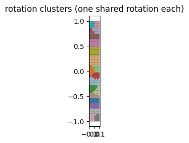
Each color is one cluster of triangles that share a single rotation in the local step. A few dozen clusters capture the bending of the whole beam, so the local step cost no longer depends on how finely the beam is meshed.
fig, ax = plt.subplots(figsize=(8, 3))
utils.setup_axes(ax, title="rotation clusters (one shared rotation each)", grid=False)
ax.tripcolor(X[:, 0], X[:, 1], T, facecolors=red.labels.astype(float),
             cmap="tab20", edgecolors="0.4", linewidth=0.3)
ax.set_aspect("equal"); fig.tight_layout(); plt.show()
5 · Rig vs. full vs. reduced#
The reduced solve reproduces the full-order secondary motion closely — the same whip and trail — while solving a system that is orders of magnitude smaller.
fig, anim = animate_panels([
    dict(states=thin(rig_states),  T=T, title="rig",                  color=RIG_C),
    dict(states=thin(full_states), T=T, title=f"full  ({full.n_rot} rot, {full.state_dim} DOF)", color=FULL_C),
    dict(states=thin(red_states),  T=T, title=f"reduced  ({red.n_rot} rot, {red.state_dim} DOF)", color=RED_C),
], suptitle="Complementary dynamics: full-order vs. fast (skinning eigenmodes)")
utils.show_video(fig, anim, "media/23_compare.mp4", fps=30)
6 · Timing: how the gap grows with resolution#
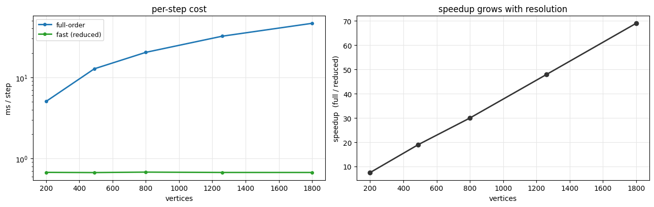
The reduced solver’s cost is set by the subspace size and the cluster count — both fixed, both independent of the mesh. So as we refine the beam, the full-order cost climbs while the reduced cost stays nearly flat, and the speedup widens.
We sweep a handful of mesh resolutions explicitly, building a fresh FullCD and ReducedCD at each
one and timing the median per-step cost.
def bench(solver, warmup=2, n=12):
    """Median ms/step for one solver under the metronome rig (after warmup)."""
    J, p0 = solver.J, solver.p0
    s = np.zeros((solver.state_dim, 1)); s_dot = np.zeros_like(s)
    p = p0.copy(); p_dot = np.zeros_like(p); ts = []
    for i in range(warmup + n):
        p_next = handle(p0, i)
        t0 = time.perf_counter()
        s_new = solver.step(s, s_dot, p, p_dot, p_next)
        dt = time.perf_counter() - t0
        s_dot = (s_new - s) / DT; p_dot = (p_next - p) / DT; s, p = s_new, p_next.copy()
        if i >= warmup: ts.append(dt)
    return 1000 * np.median(ts)

res_list = [(40, 5), (70, 7), (100, 8), (140, 9), (180, 10)]
verts, t_fulls, t_reds = [], [], []
for (w, h) in res_list:
    Xr, Tr = beam(w, h)
    tf = bench(FullCD(Xr, Tr))
    tr = bench(ReducedCD(Xr, Tr))
    verts.append(Xr.shape[0]); t_fulls.append(tf); t_reds.append(tr)
    print(f"{Xr.shape[0]:5d} verts / {Tr.shape[0]:5d} tris:  full {tf:6.1f} ms   reduced {tr:5.2f} ms   ({tf/tr:5.1f}x)")

fig, (axL, axR) = plt.subplots(1, 2, figsize=(13, 4.2))
utils.line_plot(verts, {"full-order": t_fulls, "fast (reduced)": t_reds},
                xlabel="vertices", ylabel="ms / step", markers=True, logy=True,
                colors={"full-order": FULL_C, "fast (reduced)": RED_C}, ax=axL)
axL.set_title("per-step cost")
axR.plot(verts, np.array(t_fulls) / np.array(t_reds), "-o", color="0.2", lw=2)
axR.set_xlabel("vertices"); axR.set_ylabel("speedup  (full / reduced)")
axR.set_title("speedup grows with resolution"); axR.grid(True, color="0.9")
fig.tight_layout(); plt.show()
200 verts / 312 tris: full 5.0 ms reduced 0.67 ms ( 7.5x)
490 verts / 828 tris: full 12.7 ms reduced 0.67 ms ( 19.0x)
800 verts / 1386 tris: full 20.3 ms reduced 0.68 ms ( 30.0x)
1260 verts / 2224 tris: full 32.2 ms reduced 0.67 ms ( 47.9x)
1800 verts / 3222 tris: full 46.3 ms reduced 0.67 ms ( 69.0x)
Takeaways#
Complementary dynamics = ordinary elastodynamics + one constraint. Forcing the secondary motion to be rig-orthogonal, \(J^{\top} M D\,u_c = 0\), is the whole idea. The momentum-leaking field \(D\) chooses where tissue rides with the rig versus resists it.
Full-order makes the constraint explicit through a KKT global step in an ARAP local/global solve — the same block coordinate descent as tutorials 21 & 22, with one extra constraint block. Correct, but its cost scales with the mesh.
Fast complementary dynamics moves both costs off the mesh. A rig-orthogonal skinning-eigenmode subspace makes the constraint structural (so the global solve is tiny and unconstrained), and rotation clustering fixes the number of local rotations. Per-step cost becomes essentially independent of resolution — the result reported by Benchekroun et al. (2023).
Everything here is one call away in
simkit:lbs_jacobian,diffuse_field,lbs_weight_space_constraint,skinning_eigenmodes,spectral_cubature,cluster_grouping_matrices, andsolvers.block_coord.