7 · Time Integration: Forward Euler, Backward Euler, BDF2

To animate motion we march the equations of motion in time. The integrator trades accuracy against stability and damping. We compare three on the same cantilever beam:

scheme	type	order	character
Forward Euler	explicit	1	cheap, but explodes unless dt is tiny
Backward Euler	implicit	1	rock-solid, but adds numerical damping
BDF2	implicit	2	second-order accurate, barely damps

Each implicit step minimizes the potential plus an inertia term \(\tfrac{c}{2h^2}\lVert x - \tilde x\rVert_M^2\) pulling \(x\) toward where inertia says it should go (\(\tilde x\)). We write the three steppers explicitly so the only thing that changes is \(\tilde x\) and \(c\).

%matplotlib inline
import numpy as np
import scipy as sp
import matplotlib.pyplot as plt
import simkit
from simkit.integrators import backward_euler, bdf2, forward_euler
import utils

The beam and a readable potential

BeamPotential is the static potential (elastic + pinned left edge + gravity). It composes the standard utils term helpers and sums them one per line in energy / gradient / hessian (gravity is linear, so it has no Hessian term). Each integrator layers its own inertia term on top internally.

X, T = utils.triangulated_grid(nx=14, ny=4, width=2.0, height=0.3)
n, dim = X.shape
pin_idx = np.where(X[:, 0] <= X[:, 0].min() + 1e-6)[0]

class BeamPotential:
    """Static potential: elastic + pinned left edge + gravity (no inertia)."""

    def __init__(self, X, T):
        self.p       = utils.precompute(X, T, ym=500.0, pr=0.4, rho=1.0, gravity=-9.8)
        self.psi     = utils.make_material("Neo-Hookean")
        self.pin     = utils.PenaltySpring(self.p.n, self.p.dim, 1e7).set(pin_idx, X[pin_idx])
        self.gravity = utils.Gravity(self.p.f_g)

    def energy(self, x):
        E_elastic = self.psi.energy(x, self.p)
        E_pin     = self.pin.energy(x)
        E_gravity = self.gravity.energy(x)
        return E_elastic + E_pin + E_gravity

    def gradient(self, x):
        g_elastic = self.psi.gradient(x, self.p)
        g_pin     = self.pin.gradient(x)
        g_gravity = self.gravity.gradient(x)
        return g_elastic + g_pin + g_gravity

    def hessian(self, x):
        H_elastic = self.psi.hessian(x, self.p)
        H_pin     = self.pin.hessian(x)
        return H_elastic + H_pin

pot = BeamPotential(X, T)
M = pot.p.M

The three steppers

Each takes the current state and returns the next, delegating the actual update to simkit.integrators. We carry an explicit velocity V (physical, and what the explicit method needs). The library integrators take a position history, so each wrapper just converts between the two:

• Forward Euler — forward_euler is explicit; it takes (U, V) and returns (U_next, V_next) directly.

• Backward Euler — backward_euler wants the last two positions, so we pass U and U - hV (whose backward difference is exactly V).

• BDF2 — bdf2 reconstructs two velocities from a four-level position history; we synthesize the two older positions that encode the carried V and V_prev.

NEWTON_ITERS = 30   # max Newton iterations for the implicit solves

def fe_step(U, V, h):
    """Forward (explicit) Euler via simkit.integrators.forward_euler."""
    U_next, V_next = forward_euler(U.reshape(-1, 1), V.reshape(-1, 1), pot.gradient, M, h)
    U_next = U_next.reshape(n, dim); V_next = V_next.reshape(n, dim)
    U_next[pin_idx] = X[pin_idx]; V_next[pin_idx] = 0.0      # hard-clamp the pins
    return U_next, V_next

def be_step(U, V, h):
    """Backward Euler via simkit.integrators.backward_euler.
    Pass U and (U - hV): their backward difference is exactly the velocity V."""
    U_next = backward_euler(U.reshape(-1, 1), (U - h * V).reshape(-1, 1),
                            pot.energy, pot.gradient, pot.hessian, M, h,
                            max_iter=NEWTON_ITERS, do_line_search=True).reshape(n, dim)
    V_next = (U_next - U) / h
    return U_next, V_next

def bdf2_step(U, V, U_prev, V_prev, h):
    """BDF2 via simkit.integrators.bdf2. The integrator reconstructs both
    velocities from a 4-level position history with the 2nd-order backward
    difference, so we synthesize the two older positions that encode V (at U)
    and V_prev (at U_prev)."""
    U_prev2 = 2 * h * V      - 3 * U      + 4 * U_prev     # velocity_bdf2(U, U_prev, U_prev2) = V
    U_prev3 = 2 * h * V_prev - 3 * U_prev + 4 * U_prev2    # velocity_bdf2(U_prev, U_prev2, U_prev3) = V_prev
    U_next = bdf2(U.reshape(-1, 1), U_prev.reshape(-1, 1),
                  U_prev2.reshape(-1, 1), U_prev3.reshape(-1, 1),
                  pot.energy, pot.gradient, pot.hessian, M, h,
                  max_iter=NEWTON_ITERS, do_line_search=True).reshape(n, dim)
    V_next = (3 * U_next - 4 * U + U_prev) / (2 * h)
    return U_next, V_next

Drivers that snapshot at fixed times

So we can compare runs with very different timesteps on the same time axis.

def simulate_fe(h, T_total, n_frames=60):
    sample = np.linspace(0, T_total, n_frames)
    U, V, t, si, frames = X.copy(), np.zeros_like(X), 0.0, 0, [X.copy()]
    while si < n_frames - 1:
        U, V = fe_step(U, V, h); t += h
        if not np.isfinite(U).all() or np.abs(U).max() > 1e3:        # exploded
            frames += [U.copy()] * (n_frames - len(frames)); break
        while si < n_frames - 1 and t >= sample[si + 1]:
            si += 1; frames.append(U.copy())
    return frames

def simulate_be(h, T_total, n_frames=60):
    sample = np.linspace(0, T_total, n_frames)
    U, V, t, si, frames = X.copy(), np.zeros_like(X), 0.0, 0, [X.copy()]
    while si < n_frames - 1:
        U, V = be_step(U, V, h); t += h
        while si < n_frames - 1 and t >= sample[si + 1]:
            si += 1; frames.append(U.copy())
    return frames

def simulate_bdf2(h, T_total, n_frames=60):
    sample = np.linspace(0, T_total, n_frames)
    U, V = X.copy(), np.zeros_like(X)
    U_next, V_next = be_step(U, V, h)                  # bootstrap one BE step
    U_prev, V_prev, U, V = U, V, U_next, V_next
    t, si, frames = h, 0, [X.copy()]
    while si < n_frames - 1:
        U_next, V_next = bdf2_step(U, V, U_prev, V_prev, h)
        U_prev, V_prev, U, V = U, V, U_next, V_next; t += h
        while si < n_frames - 1 and t >= sample[si + 1]:
            si += 1; frames.append(U.copy())
    return frames

Order of accuracy, measured on our beam

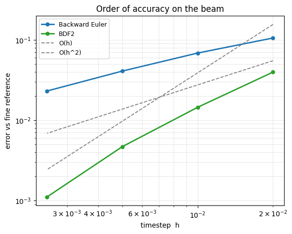
No toy oscillator: we run the beam to a fixed time and compare each scheme to a fine-timestep BDF2 reference on the same mesh. To measure order cleanly we integrate with exactly round(T/h) steps so every timestep lands at the same final time (the frame-sampling drivers above would each overshoot \(T\) by up to one step). On a log-log plot the error of an order-\(p\) method is a line of slope \(p\): Backward Euler tracks \(O(h)\); BDF2 tracks \(O(h^2)\). (Forward Euler is excluded — it needs a far smaller dt just to stay stable, as we’ll see next.)

def integrate_exact(kind, h, T_total):
    """Step EXACTLY round(T_total / h) times so every dt ends at the same time."""
    steps = int(round(T_total / h))
    U, V = X.copy(), np.zeros_like(X)
    if kind == "Backward Euler":
        for _ in range(steps):
            U, V = be_step(U, V, h)
    else:                                            # BDF2, bootstrapped with one BE step
        U_next, V_next = be_step(U, V, h)
        U_prev, V_prev, U, V = U, V, U_next, V_next
        for _ in range(2, steps + 1):
            U_next, V_next = bdf2_step(U, V, U_prev, V_prev, h)
            U_prev, V_prev, U, V = U, V, U_next, V_next
    return U

T_total = 0.5
reference = integrate_exact("BDF2", 0.0003125, T_total)          # fine BDF2 reference
hs = np.array([0.02, 0.01, 0.005, 0.0025])
errors = {
    "Backward Euler": np.array([np.linalg.norm(integrate_exact("Backward Euler", h, T_total) - reference) for h in hs]),
    "BDF2":           np.array([np.linalg.norm(integrate_exact("BDF2", h, T_total) - reference) for h in hs]),
}
for name, e in errors.items():
    print(f"{name:16s} order ~ {np.polyfit(np.log(hs), np.log(e), 1)[0]:.2f}")

fig, _ = utils.loglog_plot(hs, errors, xlabel="timestep  h", ylabel="error vs fine reference",
    colors=utils.INTEGRATOR_COLORS, ref_slopes={"O(h)": 1, "O(h^2)": 2},
    title="Order of accuracy on the beam")
plt.show()

Backward Euler   order ~ 0.73
BDF2             order ~ 1.71

Forward Euler explodes; Backward Euler doesn’t (side by side)

Explicit integration is only stable below a tiny critical timestep (CFL). At \(h = 0.008\) — a timestep Backward Euler handles without blinking — Forward Euler diverges within a few steps and flies off-screen, while Backward Euler calmly sags under gravity. This is why we use implicit integrators for stiff elasticity.

h_blow = 0.008
fe_states = simulate_fe(h_blow, 0.3, n_frames=40)
be_states = simulate_be(h_blow, 0.3, n_frames=40)
fig, anim = utils.animate_meshes_grid(
    [{"states": fe_states, "T": T, "title": f"Forward Euler  dt={h_blow}  (EXPLODES)"},
     {"states": be_states, "T": T, "title": f"Backward Euler  dt={h_blow}  (stable)"}],
    lims=((-1.3, 1.3), (-1.1, 0.5)), fps=20,
    suptitle="Same timestep: explicit blows up, implicit is fine")
utils.show_video(fig, anim, "media/07_fe_vs_be.mp4", fps=20)

Numerical damping: the timestep changes perceived stiffness

Release the beam under gravity and step Backward Euler at three (smooth, stable) timesteps — 0.001, 0.010, 0.1. Larger dt → more artificial damping → the swing dies out faster, so the material looks stiffer even though the physics is identical.

T_total = 3
dts = [0.001, 0.01, 0.1]
be_runs = [{"states": simulate_be(h, T_total, 60), "T": T, "title": f"Backward Euler  dt={h}"}
           for h in dts]
fig, anim = utils.animate_meshes_grid(be_runs, lims=((-1.2, 1.2), (-1.9, 0.5)), fps=30,
    suptitle="Backward Euler: bigger timestep -> more numerical damping")
utils.show_video(fig, anim, "media/07_be_damping.mp4", fps=30)

BDF2 barely damps

The same three timesteps with BDF2. It keeps swinging at all of them — second-order accuracy buys far less numerical dissipation than Backward Euler.

bdf2_runs = [{"states": simulate_bdf2(h, T_total, 60), "T": T, "title": f"BDF2  dt={h}"}
             for h in dts]
fig, anim = utils.animate_meshes_grid(bdf2_runs, lims=((-1.2, 1.2), (-1.9, 0.5)), fps=30,
    suptitle="BDF2: much less numerical damping at the same timesteps")
utils.show_video(fig, anim, "media/07_bdf2_damping.mp4", fps=30)

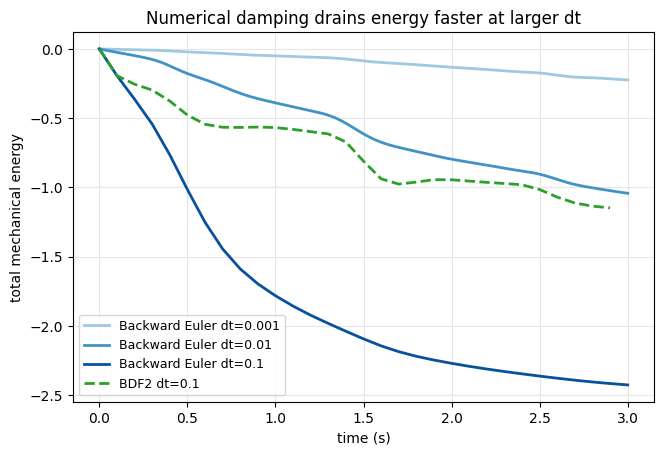
The damping, quantified: total energy bleeds away faster at bigger dt

The artificial damping isn’t just visual — it removes mechanical energy. We track the total energy (elastic + kinetic + gravitational) over time. For Backward Euler the bigger the timestep, the faster the energy drops; BDF2 (shown for the largest dt) holds onto far more of it.

def total_energy(U, V):
    E_elastic = pot.psi.energy(U.reshape(-1, 1), pot.p)
    E_kinetic = 0.5 * float(V.flatten() @ (M @ V.flatten()))
    E_gravity = pot.gravity.energy(U.reshape(-1, 1))
    return E_elastic + E_kinetic + E_gravity

def be_energy_trace(h, T_total):
    U, V = X.copy(), np.zeros_like(X)
    ts, Es = [0.0], [total_energy(U, V)]
    for s in range(int(T_total / h)):
        U, V = be_step(U, V, h); ts.append((s + 1) * h); Es.append(total_energy(U, V))
    return np.array(ts), np.array(Es)

def bdf2_energy_trace(h, T_total):
    U, V = X.copy(), np.zeros_like(X)
    Un, Vn = be_step(U, V, h); U_prev, V_prev, U, V = U, V, Un, Vn
    ts, Es = [0.0, h], [total_energy(X, np.zeros_like(X)), total_energy(U, V)]
    for s in range(2, int(T_total / h)):
        Un, Vn = bdf2_step(U, V, U_prev, V_prev, h)
        U_prev, V_prev, U, V = U, V, Un, Vn
        ts.append(s * h); Es.append(total_energy(U, V))
    return np.array(ts), np.array(Es)

fig, ax = plt.subplots(figsize=(7.5, 4.8))
shades = ["#9ecae1", "#4292c6", "#08519c"]
for h, col in zip(dts, shades):
    ts, Es = be_energy_trace(h, T_total)
    ax.plot(ts, Es, color=col, lw=2, label=f"Backward Euler dt={h}")
ts, Es = bdf2_energy_trace(0.1, T_total)
ax.plot(ts, Es, color="#2ca02c", lw=2, ls="--", label="BDF2 dt=0.1")
ax.set_xlabel("time (s)"); ax.set_ylabel("total mechanical energy")
ax.set_title("Numerical damping drains energy faster at larger dt")
ax.grid(True, color="0.9"); ax.legend(fontsize=9); plt.show()

Takeaways

• Backward Euler is order 1; BDF2 is order 2 (verified on our own beam).

• Forward Euler is explicit and explodes unless dt is tiny — implicit methods stay stable at the same dt.

• Backward Euler damps motion (and drains total energy) more as dt grows; BDF2 stays lively and conserves energy far better.