21 · Block Coordinate Descent vs. Newton — minimizing ARAP energy#
We minimize the As-Rigid-As-Possible (ARAP) elastic energy of a 2D beam. This is a pure elastostatic solve — no time, no inertia, no dynamics. The left end of the beam is clamped at rest and the right end is clamped to a rotated target, so the beam must bend round to an equilibrium. We solve the same minimization two different ways and compare iterations and wall-clock time.
Newton. Assemble the true Hessian \(H(x)\), solve \(H\,\Delta x = -\nabla E\), line-search, step. \(H\) depends on the current per-element rotations, so it changes every iteration — each step pays for a fresh sparse factorization.
Block coordinate descent (a.k.a. local/global). Introduce one auxiliary rotation \(R_t\) per triangle and alternate:
a local step — freeze \(x\), solve a per-triangle Procrustes problem, whose closed-form answer is the polar decomposition \(R_t = \mathrm{polar}(F_t)\);
a global step — freeze the rotations, minimize over \(x\). With the rotations fixed the energy is quadratic, and its minimizer solves a Poisson / Laplace-type linear system whose matrix is constant. We factorize it once and every global step is then a cheap back-substitution.
ARAP density:
It penalizes only the non-rotational part of \(F\), i.e. it behaves like a material with Poisson ratio \(\nu = 0\) (pure shear, no \(\lambda\)).
References. O. Sorkine and M. Alexa, “As-Rigid-As-Possible Surface Modeling”, SGP 2007 (the ARAP energy and its local/global solve); S. Bouaziz, S. Martin, T. Liu, L. Kavan, M. Pauly, “Projective Dynamics: Fusing Constraint Projections for Fast Simulation”, SIGGRAPH 2014 (the constant pre-factorized global solve + local projection structure).
%matplotlib inline
import time
import numpy as np
import scipy as sp
import matplotlib.pyplot as plt
import simkit
from simkit import polar_svd
from simkit.solvers import block_coord, newton_solver
import simkit.energies as energies
import utils
import warnings; warnings.filterwarnings("ignore")
np.seterr(all="ignore")           # quiet the line search's harmless overflow probes
{'divide': 'warn', 'over': 'warn', 'under': 'ignore', 'invalid': 'warn'}
A large beam, clamped at both ends#
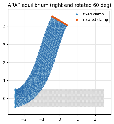
Left edge clamped at rest; the right edge clamped to its rest position rotated by \(60^\circ\) about the left-edge hinge. We enforce the clamps exactly by removing the clamped vertices’ degrees of freedom from the solve, so the only thing driving convergence is the ARAP nonlinearity itself (the per-element rotations) — not a pin spring. The constant ARAP stiffness \(L = J^\top A J\) (with \(A = \mathrm{diag}(\mathrm{vol}\cdot\mu)\otimes I\)) is the “Poisson” operator used by the global step.
X, T = utils.triangulated_grid(nx=160, ny=16, width=5.0, height=1.0)
n, dim = X.shape

# ARAP uses only mu (Poisson ratio 0); precompute gives us J and vol.
p   = utils.precompute(X, T, mu=1.0, lam=0.0)
J   = p.J
vol = p.vol
mu  = p.mu                                        # ARAP shear modulus, one row per triangle
print(f"{n} vertices, {len(T)} triangles, {n*dim} DOFs")

# constant ARAP stiffness  L = J^T A J ,  A = diag(vol * mu) (x) I
avec = np.repeat((vol.flatten() * mu.flatten()), dim * dim).reshape(-1, 1)
A = sp.sparse.diags(avec.flatten())
L = (J.T @ A @ J).tocsc()

# clamp left + right edges; rotate the right clamp by 60 deg about the left hinge
left   = np.where(X[:, 0] <= X[:, 0].min() + 1e-9)[0]
right  = np.where(X[:, 0] >= X[:, 0].max() - 1e-9)[0]
anchor = X[left].mean(axis=0)
theta  = np.deg2rad(60.0)
c, s   = np.cos(theta), np.sin(theta)
p_right = (X[right] - anchor) @ np.array([[c, -s], [s, c]]).T + anchor

# eliminate the clamped DOFs: only the free (interior) vertices are unknowns
pin_v    = np.concatenate([left, right])
pin_dof  = (pin_v[:, None] * dim + np.arange(dim)).ravel()
free_dof = np.setdiff1d(np.arange(n * dim), pin_dof)
xp = np.vstack([X[left], p_right]).reshape(-1, 1)          # clamped DOF values

L_ff = L[free_dof][:, free_dof].tocsc()
L_fp = L[free_dof][:, pin_dof].tocsc()

def make_full(xf):
    x = np.empty((n * dim, 1)); x[free_dof] = xf; x[pin_dof] = xp; return x
2560 vertices, 4770 triangles, 5120 DOFs
Block coordinate descent: one factorization, then local + global#
The whole point: \(L_{ff}\) is assembled and factorized once, in __init__.
After that the local step is a batch of per-triangle polar decompositions
(simkit.polar_svd) and the global step is a single back-substitution.
class BlockCoordARAP:
    """Local/global ARAP with a pre-factorized constant global system."""

    def __init__(self):
        self.solve   = sp.sparse.linalg.factorized(L_ff)   # the ONLY factorization
        self.rhs_pin = L_fp @ xp

    def local_step(self, xf):                 # per-triangle Procrustes: R = polar(F)
        F = (J @ make_full(xf)).reshape(-1, dim, dim)
        R, _ = polar_svd(F)
        return R.reshape(-1, 1)

    def global_step(self, xf, r):             # Poisson solve with rotations fixed
        rhs = (J.T @ (avec * r))[free_dof] - self.rhs_pin
        return self.solve(rhs).reshape(-1, 1)
Run both to convergence, recording iterations / time / state#
Shared convergence metric: the relative gradient norm \(\lVert\nabla E\rVert/\lVert\nabla E_0\rVert\)
of the full objective. We step each solver one outer iteration at a time (calling
simkit’s newton_solver and block_coord with max_iter=1) so we can record the
convergence curve and the wall-clock time. The residual evaluation used for the
plots is excluded from the timer.
RTOL = 1e-7
x0 = X.flatten().reshape(-1, 1)[free_dof]          # start from the rest pose
g0 = np.linalg.norm(gradient(x0))

def run_newton(max_iter=80):
    xf = x0.copy(); res = []; ts = []; states = [X.copy()]; t = 0.0
    for _ in range(max_iter):
        t0 = time.perf_counter()
        xf = newton_solver(xf, energy, gradient, hessian, max_iter=1, do_line_search=True)
        t += time.perf_counter() - t0
        res.append(np.linalg.norm(gradient(xf)) / g0); ts.append(t)
        states.append(make_full(xf).reshape(n, dim).copy())
        if res[-1] < RTOL: break
    return xf, np.array(res), np.array(ts), states

def run_bcd(max_iter=4000):
    bcd = BlockCoordARAP()
    xf = x0.copy(); res = []; ts = []; states = [X.copy()]; t = 0.0
    for _ in range(max_iter):
        t0 = time.perf_counter()
        xf = block_coord(xf, bcd.global_step, bcd.local_step, max_iter=1)
        t += time.perf_counter() - t0
        res.append(np.linalg.norm(gradient(xf)) / g0); ts.append(t)
        states.append(make_full(xf).reshape(n, dim).copy())
        if res[-1] < RTOL: break
    return xf, np.array(res), np.array(ts), states

xn, res_n, ts_n, states_n = run_newton()
xb, res_b, ts_b, states_b = run_bcd()
print(f"Newton              : {len(res_n):4d} iters   {1e3*ts_n[-1]:8.1f} ms   ({len(res_n)} factorizations)")
print(f"Block coord descent : {len(res_b):4d} iters   {1e3*ts_b[-1]:8.1f} ms   (1 factorization)")
print(f"per iteration       : Newton {1e3*ts_n[-1]/len(res_n):6.2f} ms   |   BCD {1e3*ts_b[-1]/len(res_b):6.2f} ms")
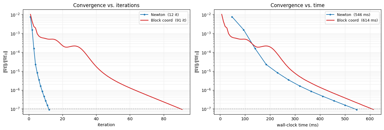
Newton              :   12 iters      546.4 ms   (12 factorizations)
Block coord descent :   91 iters      614.1 ms   (1 factorization)
per iteration       : Newton  45.54 ms   |   BCD   6.75 ms
Convergence: iterations vs. wall-clock time#
Left: residual per outer iteration. Right: residual vs. elapsed time. Newton’s search direction uses curvature, so it needs far fewer iterations; block coordinate descent needs many more (its constant rest-pose metric is a first-order model of the curvature), but each iteration is several times cheaper because it reuses one factorization. The two panels make the trade-off explicit for this mesh.
fig, ax = plt.subplots(1, 2, figsize=(13, 4.5))
ax[0].semilogy(np.arange(1, len(res_n)+1), res_n, "-o", ms=3, color="#1f77b4", label=f"Newton  ({len(res_n)} it)")
ax[0].semilogy(np.arange(1, len(res_b)+1), res_b, "-",  lw=1.8, color="#d62728", label=f"Block coord  ({len(res_b)} it)")
ax[1].semilogy(1e3*ts_n, res_n, "-o", ms=3, color="#1f77b4", label=f"Newton  ({1e3*ts_n[-1]:.0f} ms)")
ax[1].semilogy(1e3*ts_b, res_b, "-",  lw=1.8, color="#d62728", label=f"Block coord  ({1e3*ts_b[-1]:.0f} ms)")
for a, xl in zip(ax, ["iteration", "wall-clock time (ms)"]):
    a.axhline(RTOL, color="0.6", ls="--", lw=1); a.set_xlabel(xl)
    a.set_ylabel(r"$\|\nabla E\| / \|\nabla E_0\|$")
    a.grid(True, which="both", color="0.92"); a.legend(fontsize=9)
ax[0].set_title("Convergence vs. iterations"); ax[1].set_title("Convergence vs. time")
fig.tight_layout(); fig.savefig("media/21_convergence.png", dpi=130, bbox_inches="tight"); plt.show()
The equilibrium shape#
Both solvers reach the same ARAP minimizer (the rest beam is ghosted in gray).
U = make_full(xn).reshape(n, dim)
lims = utils.auto_limits([X, U], pad=0.4)
fig, axx = plt.subplots(figsize=(7.5, 4.8))
utils.setup_axes(axx, *lims, title="ARAP equilibrium (right end rotated 60 deg)")
utils.PolyMeshArtist(axx, X, T, facecolor="#efefef", edgecolor="#cfcfcf", lw=0.3)   # rest ghost
utils.PolyMeshArtist(axx, U, T, facecolor="#9ecae1", edgecolor="#08519c", lw=0.3)
axx.scatter(X[left][:, 0], X[left][:, 1], s=12, color="#3182bd", zorder=5, label="fixed clamp")
axx.scatter(p_right[:, 0], p_right[:, 1], s=12, color="#e6550d", zorder=5, label="rotated clamp")
axx.legend(loc="upper right", fontsize=9); plt.show()
Watching each solver converge#
One frame per (sub-sampled) iteration. Block coordinate descent sweeps the beam into the right gross shape almost immediately, then spends its long tail polishing; Newton takes a few big curvature-aware steps.
def thin(states, target=50):
    k = max(1, len(states) // target); idx = list(range(0, len(states), k))
    if idx[-1] != len(states) - 1: idx.append(len(states) - 1)
    return [states[i] for i in idx]

clamp_pts = np.vstack([X[left], p_right])
lims = utils.auto_limits([X, make_full(xn).reshape(n, dim)], pad=0.4)
fig, anim = utils.animate_mesh(thin(states_b), T, lims=lims, fps=12,
    title="Block coordinate descent (local/global) converging", pin_pts=clamp_pts)
utils.show_video(fig, anim, "media/21_bcd.mp4", fps=12)
fig, anim = utils.animate_mesh(states_n, T, lims=lims, fps=5,
    title="Newton converging", pin_pts=clamp_pts)
utils.show_video(fig, anim, "media/21_newton.mp4", fps=5)
Takeaways#
Same minimizer, two cost structures. Newton spends a lot per iteration (assemble a state-dependent Hessian, re-factorize, line-search) but converges in very few iterations thanks to curvature. Block coordinate descent factorizes once and every iteration is a parallel batch of polar decompositions plus a single back-substitution — cheap, but it needs many more of them because the constant rest-pose metric only models the curvature to first order.
Read the two plots together. Iteration count and wall-clock time tell different stories; the right-hand panel is the one that matters in practice, and where it crosses depends on the mesh size, the accuracy you demand, and the cost of a factorization (which grows fast with problem size, especially in 3D).
The structure is the lesson.
local_step= per-element Procrustes (polar_svd);global_step= one prefactored Poisson solve. That “project, then solve a constant system” pattern is exactly projective dynamics, and it is what the next tutorial reuses for mass-springs.