17 · Skinning Eigenmodes: a Subspace that Can Rotate#
A high-resolution beam is accurate but slow (tutorial 10): every Backward-Euler step solves a sparse system as big as the mesh. Reduced-order modeling escapes this by restricting the motion to a small subspace
and solving for the \(r\) subspace coordinates \(z\) instead of all \(n\,\text{dim}\) vertex DOFs. The basis \(B\) is built once, offline. The question is which basis — and the answer hinges on one thing: can the subspace rotate?
Linear Modal Analysis (LMA) uses the lowest vibration modes as displacement columns: \(x = X + B_{\text{lma}}z\). Fast, but a sum of fixed displacement fields is linear in \(z\) — and rotation is not a linear function of position. LMA literally cannot turn the rest shape.
Skinning eigenmodes use the same Laplacian eigenvectors as skinning weights and attach a small affine transform to each: \(x = B_{\text{skin}}z\), where \(z\) stacks per-bone \(2\times3\) transforms. Affine transforms contain rotation, so this subspace turns the shape exactly — for the same solve cost.
We will (1) feel the cost of the full solve, (2) show the subspace shrinks the solve (not the integration), (3) watch a cantilever sag and see LMA fail to rotate while skinning tracks the full reference, and (4) rotate the rest shape a full turn and measure each subspace’s reconstruction error.
%matplotlib inline
import time
import numpy as np
import scipy as sp
import scipy.sparse as sps
import matplotlib.pyplot as plt
from matplotlib.animation import FuncAnimation

import simkit
from simkit.solvers import newton_solver
import utils

import warnings
from scipy.linalg import LinAlgWarning
warnings.filterwarnings("ignore", category=LinAlgWarning)   # stiff pin -> benign ill-conditioning

FULL_C = "#d62728"   # full-space (reference / "slow")
LMA_C  = "#1f77b4"   # linear modal analysis
SKIN_C = "#2ca02c"   # skinning eigenmodes
A neo-Hookean beam, sagging under gravity, with inertia#
We reuse the cantilever of tutorial 10 but now make it dynamic: each step is one Backward-Euler solve of the incremental potential
with momentum target \(\tilde x = 2x_n - x_{n-1}\) (i.e. \(x_n + h v_n\)), full-order neo-Hookean elasticity, gravity, and a stiff penalty clamping the left wall. BeamSim wraps the mesh, the precomputed operators, and a single Newton step — and takes an optional subspace \((B, q)\). With \(B = I\) it solves the full per-vertex system; with a reduced \(B\) it solves for \(z\) via the Galerkin projection \(B^{\top} g\), \(B^{\top} H B\) (full integration — we evaluate the real energy and project, no cubature).
The class follows the standardized recipe: utils.precompute for \(J/\text{vol}/\mu/\text{lam}/M/f_g\), a utils.PenaltySpring for the wall pin, and a utils.Inertia for backward-Euler. Each energy/gradient/Hessian term is built on its own line on the full \(x = Bz+q\), then the gradient/Hessian are projected with \(B^{\top}\).
class BeamSim:
    """Backward-Euler neo-Hookean cantilever. Optional subspace x = B z + q."""

    def __init__(self, nx, ny, ym=3000.0, pr=0.4, rho=1.0, h=2e-2,
                 B=None, q=None, K_pin=1e7, width=4.0, height=0.5):
        self.X, self.T = utils.triangulated_grid(nx, ny, width=width, height=height)
        self.p   = utils.precompute(self.X, self.T, ym=ym, pr=pr, rho=rho, gravity=-9.8)
        self.n, self.dim = self.p.n, self.p.dim
        self.h   = h

        self.psi     = utils.make_material("Neo-Hookean")   # full-order elastic term
        self.gravity = utils.Gravity(self.p.f_g)
        self.inertia = utils.Inertia(self.p.M, h)
        self.Mk      = self.p.M                              # mass in the subspace projection

        pin_idx = np.where(self.X[:, 0] <= self.X[:, 0].min() + 1e-6)[0]
        self.pin_idx = pin_idx
        self.pin = utils.PenaltySpring(self.n, self.dim, K_pin).set(pin_idx, self.X[pin_idx])

        # subspace: x = B z + q   (B = identity => full space)
        self.B = sps.identity(self.n * self.dim).tocsc() if B is None else B
        self.q = np.zeros((self.B.shape[0], 1)) if q is None else q.reshape(-1, 1)
        self.tip = int(np.argmax(self.X[:, 0]))

    def _x(self, z):  return self.B @ z + self.q

    def energy(self, z):
        x = self._x(z)
        E_inertia = self.inertia.energy(x)
        E_elastic = self.psi.energy(x, self.p)
        E_gravity = self.gravity.energy(x)
        E_pin     = self.pin.energy(x)
        return E_inertia + E_elastic + E_gravity + E_pin

    def gradient(self, z):
        x = self._x(z)
        g_elastic = self.B.T @ self.psi.gradient(x, self.p)
        g_gravity = self.B.T @ self.gravity.gradient(x)
        g_pin     = self.B.T @ self.pin.gradient(x)
        g_inertia = self.B.T @ self.inertia.gradient(x)
        return g_elastic + g_gravity + g_pin + g_inertia

    def hessian(self, z):
        x = self._x(z)
        H_elastic = self.B.T @ (self.psi.hessian(x, self.p) @ self.B)
        H_pin     = self.B.T @ (self.pin.hessian(x) @ self.B)
        H_inertia = self.B.T @ (self.inertia.hessian(x) @ self.B)
        return H_elastic + H_pin + H_inertia

    def rest_z(self):
        """Subspace coordinates of the rest shape (mass-weighted projection)."""
        return simkit.project_into_subspace(self.X.reshape(-1, 1) - self.q, self.B, M=self.Mk)

    def step(self, z, z_prev, iters=30):
        """One Backward-Euler step; Newton with line search (required for stability)."""
        x_n = self.B @ z + self.q
        v_n = (x_n - (self.B @ z_prev + self.q)) / self.h
        self.inertia.update(x_n, v_n)                        # x_tilde = x_n + h v_n
        return newton_solver(z.copy(), self.energy, self.gradient, self.hessian,
                             max_iter=iters, do_line_search=True)

    def simulate(self, n_steps=80):
        """Drop from rest under gravity; return per-step poses and tip height."""
        z = self.rest_z(); z_prev = z.copy()
        states, tip_y = [self._x(z).reshape(self.n, self.dim)], [self.X[self.tip, 1]]
        for _ in range(n_steps):
            z, z_prev = self.step(z, z_prev), z
            U = self._x(z).reshape(self.n, self.dim)
            states.append(U); tip_y.append(U[self.tip, 1])
        return np.array(states), np.array(tip_y)
The full solve is slow#
A genuinely high-resolution beam (here ~3600 vertices, ~7200 DOFs). We assemble one Backward-Euler system at a deformed state and time the linear solve alone and the gradient + Hessian evaluation alone — the two halves of every Newton iteration. The solve is the part that grows with mesh size.
hi = BeamSim(120, 30)                       # high-res "slow" beam
print(f"high-res mesh: {hi.n} vertices, {hi.T.shape[0]} triangles, {hi.n*hi.dim} DOFs")

# a representative deformed state + a momentum target, so the system is realistic
rng = np.random.RandomState(0)
x_def = (hi.X + 0.05 * rng.randn(hi.n, hi.dim)).reshape(-1, 1)
hi.inertia.update(hi.X.reshape(-1, 1), np.zeros((hi.n * hi.dim, 1)))
z_def = x_def                                # full space: z == x

def time_call(fn, inner=1, rep=7):
    """Min over `rep` batches of `inner` calls each -> robust for sub-ms timings."""
    best = float("inf")
    for _ in range(rep):
        t0 = time.perf_counter()
        for _ in range(inner):
            fn()
        best = min(best, (time.perf_counter() - t0) / inner)
    return best

# eval = assemble gradient + Hessian; solve = the linear system, timed in isolation
def assemble_full():
    return hi.hessian(z_def).tocsc(), hi.gradient(z_def)
H_full, g_full = assemble_full()
t_eval_full  = time_call(assemble_full, inner=1, rep=5)
t_solve_full = time_call(lambda: sps.linalg.spsolve(H_full, -g_full), inner=3, rep=7)
print(f"full-space eval (grad+Hess): {t_eval_full*1e3:7.1f} ms")
print(f"full-space linear solve    : {t_solve_full*1e3:7.1f} ms")
high-res mesh: 3600 vertices, 6902 triangles, 7200 DOFs
full-space eval (grad+Hess):    23.0 ms
full-space linear solve    :    12.7 ms
Two subspaces, built once#
simkit.linear_modal_analysis returns the lowest \(k\) vibration modes as a displacement basis \(B_{\text{lma}}\in\mathbb{R}^{n\,\text{dim}\times k}\). simkit.skinning_eigenmodes returns the Laplacian eigenvector weights \(W\) and the corresponding LBS Jacobian \(B_{\text{skin}}\in\mathbb{R}^{n\,\text{dim}\times 6k}\) (each of the \(k\) modes carries a \(2\times3\) affine transform = 6 DOFs in 2D). Same \(k\), but skinning spends its extra columns buying rotation.
k = 12
E_lma,  B_lma  = simkit.linear_modal_analysis(hi.X, hi.T, k*6)
W, E_s, B_skin = simkit.skinning_eigenmodes(hi.X, hi.T, k)
B_lma  = np.asarray(B_lma)
B_skin = np.asarray(B_skin)
print(f"k = {k} modes")
print(f"  LMA  basis: {B_lma.shape[1]:3d} columns  (k displacement modes)")
print(f"  SKIN basis: {B_skin.shape[1]:3d} columns  (k modes x 6 affine DOFs)")

# show three skinning weight fields W (the partition the affine bones blend over)
fig, axes = plt.subplots(1, 3, figsize=(13, 2.2))
for ax, j in zip(axes, [1, 4, 8]):
    tc = ax.tripcolor(hi.X[:, 0], hi.X[:, 1], hi.T, W[:, j], shading="gouraud", cmap="RdBu")
    ax.set_aspect("equal"); ax.axis("off"); ax.set_title(f"skinning weight  $W_{{{j}}}$")
fig.suptitle("skinning eigenmode weights = Laplacian eigenvectors")
plt.show()
k = 12 modes
  LMA  basis:  72 columns  (k displacement modes)
  SKIN basis:  72 columns  (k modes x 6 affine DOFs)

The subspace shrinks the solve, not the integration#
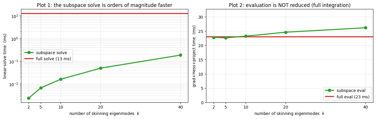
Every Newton iteration is evaluate (assemble gradient + Hessian) then solve (one linear system). With full integration the reduced model still evaluates the real neo-Hookean energy on every element and projects it (\(B^{\top}g\), \(B^{\top}HB\)), so its eval cost is unchanged. What collapses is the solve: from an \(n\,\text{dim}\times n\,\text{dim}\) sparse system to a tiny dense \(r\times r\) one.
Plot 1 — linear-solve time vs. number of skinning eigenmodes, with the full-space solve drawn as a red line towering above. Plot 2 — the eval (grad+Hess+projection) time, full vs. subspace: essentially equal, because the integration is not reduced.
mode_counts = [2, 5, 10, 20, 40]
solve_red, eval_red = [], []
for kk in mode_counts:
    _, _, Bk = simkit.skinning_eigenmodes(hi.X, hi.T, kk)
    Bk = np.asarray(Bk)
    def assemble_red(Bk=Bk):
        x = x_def
        g = hi.inertia.gradient(x)
        g = g + hi.psi.gradient(x, hi.p)
        g = g + hi.gravity.gradient(x) + hi.pin.gradient(x)
        H = hi.inertia.hessian(x) + hi.pin.hessian(x)
        H = H + hi.psi.hessian(x, hi.p)
        return Bk.T @ (H @ Bk), Bk.T @ g
    Hz, gz = assemble_red(Bk)                                  # assemble once
    te = time_call(assemble_red, inner=1, rep=5)               # eval (full integration + projection)
    ts = time_call(lambda Hz=Hz, gz=gz: np.linalg.solve(Hz, -gz), inner=200, rep=7)  # solve, isolated
    eval_red.append(te * 1e3); solve_red.append(ts * 1e3)
    print(f"  skinning k={kk:2d} (r={Bk.shape[1]:3d}): solve {solve_red[-1]:8.5f} ms   eval {eval_red[-1]:6.1f} ms")

mc = np.array(mode_counts)
fig, (axL, axR) = plt.subplots(1, 2, figsize=(13, 4.2))

axL.plot(mc, solve_red, "-o", color=SKIN_C, lw=2.5, ms=7, label="subspace solve", zorder=3)
axL.axhline(t_solve_full * 1e3, color=FULL_C, lw=2.5, ls="-", zorder=4,
            label=f"full solve ({t_solve_full*1e3:.0f} ms)")
axL.set_yscale("log"); axL.set_xticks(mc)
axL.set_xlabel("number of skinning eigenmodes  $k$"); axL.set_ylabel("linear-solve time  (ms)")
axL.set_title("Plot 1: the subspace solve is orders of magnitude faster")
axL.legend(loc="center left"); axL.grid(True, which="both", color="0.9")

axR.plot(mc, eval_red, "-o", color=SKIN_C, lw=2.5, ms=7, label="subspace eval", zorder=3)
axR.axhline(t_eval_full * 1e3, color=FULL_C, lw=2.5, label=f"full eval ({t_eval_full*1e3:.0f} ms)")
axR.set_xticks(mc); axR.set_ylim(0, max(t_eval_full * 1e3, max(eval_red)) * 1.25)
axR.set_xlabel("number of skinning eigenmodes  $k$"); axR.set_ylabel("grad+Hess+project time  (ms)")
axR.set_title("Plot 2: evaluation is NOT reduced (full integration)")
axR.legend(loc="lower right"); axR.grid(True, color="0.9")
fig.tight_layout(); fig.savefig("media/17_timing.png", dpi=130, bbox_inches="tight"); plt.show()
  skinning k= 2 (r= 12): solve  0.00234 ms   eval   22.8 ms
  skinning k= 5 (r= 30): solve  0.00655 ms   eval   22.6 ms
skinning k=10 (r= 60): solve 0.01577 ms eval 23.2 ms
skinning k=20 (r=120): solve 0.04886 ms eval 24.6 ms
skinning k=40 (r=240): solve 0.18301 ms eval 26.1 ms
Fast solve — but does it look right?#
Cost is only half the story. We now run the same dynamic sag in all three spaces on a softer beam (so the free end swings through a large angle) and play them side by side: the full-order reference, LMA, and skinning. Watch the tip.
We build the three simulators explicitly — full (\(B=I\)), LMA (\(x = X + B_{\text{lma}}z\), so \(q = X\)), and skinning (\(x = B_{\text{skin}}z\), so \(q = 0\)) — and run each from rest.
nx, ny = 50, 11
full = BeamSim(nx, ny)
Xs, Ts = full.X, full.T
El, Bl = simkit.linear_modal_analysis(Xs, Ts, k)
Ws, Es2, Bs = simkit.skinning_eigenmodes(Xs, Ts, k)
lma  = BeamSim(nx, ny, B=np.asarray(Bl), q=Xs.reshape(-1, 1))     # x = X + B z
skin = BeamSim(nx, ny, B=np.asarray(Bs))                          # x = B z

st_full, ty_full = full.simulate(80)
st_lma,  ty_lma  = lma.simulate(80)
st_skin, ty_skin = skin.simulate(80)

def area_ratio(U):
    a = lambda V: 0.5 * ((V[Ts[:,1],0]-V[Ts[:,0],0])*(V[Ts[:,2],1]-V[Ts[:,0],1])
                       -  (V[Ts[:,1],1]-V[Ts[:,0],1])*(V[Ts[:,2],0]-V[Ts[:,0],0]))
    r = a(U) / a(Xs); return r.min(), r.max()
print(f"final tip height:  full {ty_full[-1]:+.2f}   LMA {ty_lma[-1]:+.2f}   skin {ty_skin[-1]:+.2f}")
print(f"LMA  under-rotates: tip only reaches {abs(ty_lma[-1]/ty_full[-1])*100:.0f}% of the full droop")
print(f"area ratio [min,max]:  full {tuple(round(v,2) for v in area_ratio(st_full[-1]))}"
      f"   LMA {tuple(round(v,2) for v in area_ratio(st_lma[-1]))}"
      f"   skin {tuple(round(v,2) for v in area_ratio(st_skin[-1]))}")

panels = [
    {"states": st_full, "T": Ts, "title": f"full  ({full.n*full.dim} DOFs)"},
    {"states": st_lma,  "T": Ts, "title": f"LMA  ({Bl.shape[1]} DOFs)  -- can't rotate"},
    {"states": st_skin, "T": Ts, "title": f"skinning  ({Bs.shape[1]} DOFs)  -- rotates"},
]
fig, anim = utils.animate_meshes_grid(panels, lims=((-2.5, 2.5), (-4.2, 0.6)), fps=20,
                                      suptitle="same sag in three spaces: LMA stalls, skinning tracks the full beam")
utils.show_video(fig, anim, "media/17_dynamics.mp4", fps=20)
final tip height:  full -3.48   LMA -0.56   skin -3.01
LMA  under-rotates: tip only reaches 16% of the full droop
area ratio [min,max]:  full (np.float64(0.81), np.float64(1.23))   LMA (np.float64(0.98), np.float64(1.02))   skin (np.float64(0.82), np.float64(1.17))
The decisive test: rotate the rest shape a full turn#
The dynamics hinted at it; this proves it. Take the rest beam, rotate it by \(\theta\) through a full \(360^\circ\), and ask each subspace to reproduce that rigid rotation: project the rotated mesh into the subspace in the mass norm (project_into_subspace with \(M\)), reconstruct \(x = Bz+q\), and measure the relative error \(\lVert Bz+q - x_\theta\rVert_M / \lVert x_\theta\rVert_M\).
A pure rotation is a rigid motion — no strain, the lowest-energy thing a body can do — yet LMA cannot represent it: its columns are fixed displacement fields, and the error grows with the angle, peaking when the shape is upside-down. Skinning carries a rotation in every bone’s affine block, so it reproduces the turn to machine precision at every angle.
Mk = sps.kron(simkit.massmatrix(Xs, Ts), sps.identity(2)).tocsc()
q_lma  = Xs.reshape(-1, 1)
q_skin = np.zeros((Xs.size, 1))
xr = Xs.reshape(-1, 1)

def reconstruct(y, B, q):
    z = simkit.project_into_subspace(y - q, B, M=Mk)
    return B @ z + q

def rel_err(rec, y):
    d = rec - y
    return float(np.sqrt((d.T @ Mk @ d)[0, 0]) / np.sqrt((y.T @ Mk @ y)[0, 0]))

angles = np.linspace(0, 360, 73)
targets, rec_lma, rec_skin, err_lma, err_skin = [], [], [], [], []
for deg in angles:
    th = np.deg2rad(deg)
    R = np.array([[np.cos(th), -np.sin(th)], [np.sin(th), np.cos(th)]])
    y = (Xs @ R.T).reshape(-1, 1)
    rl = reconstruct(y, np.asarray(Bl), q_lma)
    rsk = reconstruct(y, np.asarray(Bs), q_skin)
    targets.append(y.reshape(-1, 2)); rec_lma.append(rl.reshape(-1, 2)); rec_skin.append(rsk.reshape(-1, 2))
    err_lma.append(rel_err(rl, y)); err_skin.append(rel_err(rsk, y))
err_lma, err_skin = np.array(err_lma), np.array(err_skin)
print(f"LMA  reconstruction error: 0 -> {err_lma.max():.3f} (peak at 180 deg) -> 0")
print(f"skin reconstruction error: max {err_skin.max():.1e}  (machine zero, all angles)")
LMA  reconstruction error: 0 -> 0.342 (peak at 180 deg) -> 0
skin reconstruction error: max 7.2e-10  (machine zero, all angles)
fig, (axA, axB, axR) = plt.subplots(1, 3, figsize=(15, 4.4),
                                    gridspec_kw={"width_ratios": [1, 1, 1.15]})

# --- panel A: LMA reconstruction (target ghosted underneath) ---
utils.setup_axes(axA, (-3.0, 3.0), (-3.0, 3.0), title="LMA reconstruction")
mtA = utils.PolyMeshArtist(axA, targets[0], Ts, facecolor="0.9", edgecolor="0.65", lw=0.4)
ml  = utils.PolyMeshArtist(axA, rec_lma[0], Ts, facecolor="none", edgecolor=LMA_C, lw=1.0)
axA.plot([], [], color="0.65", lw=2, label="target (rotated rest)")
axA.plot([], [], color=LMA_C, lw=2, label="LMA")
axA.legend(loc="upper right", fontsize=8)

# --- panel B: skinning reconstruction (target ghosted underneath) ---
utils.setup_axes(axB, (-3.0, 3.0), (-3.0, 3.0), title="skinning reconstruction")
mtB = utils.PolyMeshArtist(axB, targets[0], Ts, facecolor="0.9", edgecolor="0.65", lw=0.4)
msk = utils.PolyMeshArtist(axB, rec_skin[0], Ts, facecolor="none", edgecolor=SKIN_C, lw=1.0)
axB.plot([], [], color="0.65", lw=2, label="target (rotated rest)")
axB.plot([], [], color=SKIN_C, lw=2, label="skinning")
axB.legend(loc="upper right", fontsize=8)

# --- panel R: reconstruction error vs rotation angle ---
trace = utils.TracePlot(axR, angles, {"LMA": err_lma, "skinning": err_skin},
                        colors={"LMA": LMA_C, "skinning": SKIN_C},
                        xlabel="rest-shape rotation  (deg)", ylabel="reconstruction error  (mass norm)",
                        title="LMA error peaks upside-down; skinning stays ~0")

def update(i):
    mtA.update(targets[i]); ml.update(rec_lma[i])
    mtB.update(targets[i]); msk.update(rec_skin[i])
    trace.update(i)
    return ()

anim = FuncAnimation(fig, update, frames=len(angles), interval=1000/18, blit=False)
fig.savefig("media/17_rotation_error.png", dpi=130, bbox_inches="tight")
utils.show_video(fig, anim, "media/17_rotation_error.mp4", fps=18)
Does adding modes fix it? Integrate the error over a full turn#
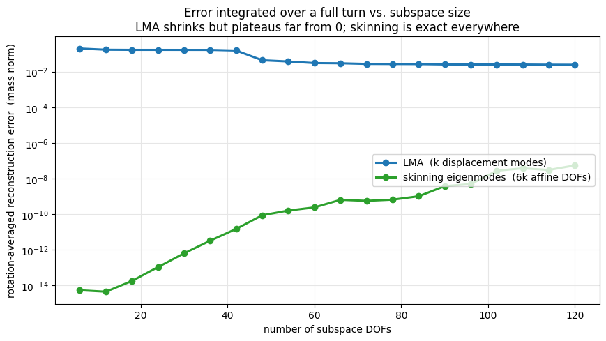
The curve above is for one fixed basis. The real question is how the error behaves as we grow the subspace. For 20 different subspace sizes we integrate the reconstruction error over the entire \(360^\circ\) rotation — its average over all angles — and plot it against the number of subspace DOFs.
Adding modes lets LMA chase the rotation a little better, so its turn-averaged error decreases — but a linear basis can never contain a rotation, so the error plateaus far from zero no matter how many modes we spend. Skinning carries a rotation inside every bone’s affine block, so it is exact at every size — even a single bone (6 DOFs) reproduces the full turn to machine precision.
# integrate the reconstruction error over a full 360-degree turn, for 20 subspace sizes
mode_range = np.arange(1, 21)
ang_int = np.linspace(0, 360, 49)
Rg = [np.array([[np.cos(t), -np.sin(t)], [np.sin(t), np.cos(t)]]) for t in np.deg2rad(ang_int)]
Yg = [(Xs @ R.T).reshape(-1, 1) for R in Rg]
yn = np.array([float(np.sqrt((y.T @ Mk @ y)[0, 0])) for y in Yg])

def turn_avg_error(B, q):
    """Reconstruction error averaged over the whole 360-degree rotation sweep."""
    B = np.asarray(B); BMB = B.T @ (Mk @ B)
    errs = []
    for y, ym in zip(Yg, yn):
        z = np.linalg.solve(BMB, B.T @ (Mk @ (y - q)))
        d = B @ z + q - y
        errs.append(float(np.sqrt((d.T @ Mk @ d)[0, 0])) / ym)
    return float(np.mean(errs))

dof_lma, dof_skin, ei_lma, ei_skin = [], [], [], []
for kk in mode_range:
    _, Bl    = simkit.linear_modal_analysis(Xs, Ts, kk*6)
    _, _, Bs = simkit.skinning_eigenmodes(Xs, Ts, kk)
    dof_lma.append(Bl.shape[1]);  ei_lma.append(turn_avg_error(Bl, Xs.reshape(-1, 1)))
    dof_skin.append(Bs.shape[1]); ei_skin.append(turn_avg_error(Bs, np.zeros((Xs.size, 1))))
print(f"LMA : up to {dof_lma[-1]:3d} DOFs -> turn-averaged error plateaus at {min(ei_lma):.3f} (never rotates)")
print(f"skin: up to {dof_skin[-1]:3d} DOFs -> turn-averaged error max {max(ei_skin):.1e} (exact at every size)")

fig, ax = plt.subplots(figsize=(8.8, 5.0))
ax.plot(dof_lma,  ei_lma,  "-o", color=LMA_C,  lw=2.2, ms=6, label="LMA  (k displacement modes)")
ax.plot(dof_skin, ei_skin, "-o", color=SKIN_C, lw=2.2, ms=6, label="skinning eigenmodes  (6k affine DOFs)")
ax.set_yscale("log")
ax.set_xlabel("number of subspace DOFs"); ax.set_ylabel("rotation-averaged reconstruction error  (mass norm)")
ax.set_title("Error integrated over a full turn vs. subspace size\nLMA shrinks but plateaus far from 0; skinning is exact everywhere")
ax.grid(True, which="both", color="0.9"); ax.legend(loc="center right")
fig.tight_layout(); fig.savefig("media/17_integrated_error.png", dpi=130, bbox_inches="tight"); plt.show()
LMA : up to 120 DOFs -> turn-averaged error plateaus at 0.024 (never rotates)
skin: up to 120 DOFs -> turn-averaged error max 5.4e-08 (exact at every size)
Takeaways#
A subspace \(x=Bz+q\) replaces an \(n\,\text{dim}\)-DOF solve with an \(r\)-DOF one. With full integration (no cubature) the gradient/Hessian still cost the full assembly — the subspace shrinks the linear solve, which is the part that explodes with resolution (Plots 1–2).
Linear Modal Analysis is a sum of fixed displacement fields: linear in \(z\). Rotation is nonlinear in position, so it lives outside the LMA subspace — the reconstruction error of a rotated rest shape grows with the angle and peaks at \(180^\circ\). In dynamics this shows up as a free end that refuses to swing.
Skinning eigenmodes attach an affine transform (which contains rotation) to each Laplacian-eigenvector weight field, so the subspace reproduces rigid rotation to machine precision at every angle — and tracks the full-order sag where LMA stalls.
Rule of thumb: if the motion rotates — cantilevers, tails, tentacles, characters — use a rotation-aware subspace like skinning eigenmodes.
This extends the SimKit tutorials into reduced-order modeling: same neo-Hookean physics as tutorials 3–10, now solved in a handful of coordinates.